Waning vaccine efficacy on susceptibility

In this article, I examined the process of modifying the disease transmission model (for instance, the \(SEIR\) model) to include vaccination and the waning of vaccine-induced immunity as it might happen in a clinical trial. A straightforward method to represent this involves assuming vaccinated individuals (i.e., those in the vaccinated, \(V\), compartment) possess partial immunity and subsequently transition back to the susceptible, \(S\), compartment. This approach effectively simulates the diminishing effectiveness of vaccines using two parameters. I focus on determining these parameters through the analysis of existing vaccine efficacy data, utilizing the typhoid vaccine clinical trial as a case study. The adaptation of the model to account for the progressive reduction in vaccine-derived immunity across various compartments was conducted prior post.

Vaccine efficacy data

Vaccine efficacy data come from a clinical trial conducted in Malawi from 2018 through 2023, for which the detailed information is available in the study.

# df <- data.frame(year=c(1,2), efficacy=c(83.4,73.0)) # Shakya (2021) Lancet Glob Health

# vaccine efficacy cumulative over the four years
# Patel (2024) Lancet
tab2_vitt <- data.frame(group = "Vi-TT",
                   age = c("<2yo","2-4yo",">=5yo","all_ITT","all_PP"),
                   person_years = c(6586,15007,38907,60500,59942), 
                   typhoid_culture = c(4,5,15,24,22),
                   IR_obs = c(60.7,33.3,38.6,39.7,36.7),
                   VE_obs = c(70.6,79.6,79.3,78.3,80.0))

tab2_mena <- data.frame(group = "MenA",
                   age = c("<2yo","2-4yo",">=5yo","all_ITT","all_PP"),
                   person_years = c(6773,15297,38151,60220,59662), 
                   typhoid_culture = c(14,25,71,110,109),
                   IR_obs = c(206.7,163.4,186.1,182.7,182.7),
                   VE_obs = NA)

tab2 <- rbind(tab2_vitt, tab2_mena)
# Check the sanity of the data
tab2$IR_cal <- round(tab2$typhoid_culture/tab2$person_years*1e5, digits=1)
tab2$IR_cal == tab2$IR_obs

 [1] TRUE TRUE TRUE TRUE TRUE TRUE TRUE TRUE TRUE TRUE

tab2$VE_cal <- NA
tab2[tab2$group == "Vi-TT",]$VE_cal <- 
  round(100*(1 - tab2[tab2$group == "Vi-TT",]$IR_cal/
               tab2[tab2$group == "MenA",]$IR_cal),digits=1) 
tab2$VE_cal == tab2$VE_obs

 [1]  TRUE  TRUE  TRUE  TRUE FALSE    NA    NA    NA    NA    NA

tab3_vitt <- data.frame(group = "Vi-TT",
                   age = "all_ITT",
                   person_years = c(14058,28104,42135,56121,60500),
                   year_since_vacc = c(1,2,3,4,4.61),
                   typhoid_culture = c(6,12,15,23,24),
                   IR_obs = c(42.7,42.7,35.6,41.0,39.7),
                   VE_obs=c(83.4,80.7,80.1,77.1,78.3))
tab3_mena <- data.frame(group = "MenA",
                   age = "all_ITT",
                   person_years = c(14036,28021,41983,55889,60220),
                   year_since_vacc = c(1,2,3,4,4.61),
                   typhoid_culture = c(36,62,75,100,110),
                   IR_obs = c(256.5,221.3,178.6,178.9,182.7),
                   VE_obs = NA)
tab3 <- rbind(tab3_vitt, tab3_mena)
# Check the sanity of the data
tab3$IR_cal <- round(tab3$typhoid_culture/tab3$person_years*1e5, digits=1)
tab3$VE_cal <- NA
tab3[tab3$group == "Vi-TT",]$VE_cal <- 
  round(100*(1 - tab3[tab3$group == "Vi-TT",]$IR_cal/
               tab3[tab3$group == "MenA",]$IR_cal),digits=1) 
tab3$VE_cal == tab3$VE_obs

 [1] TRUE TRUE TRUE TRUE TRUE   NA   NA   NA   NA   NA

Model of typhoid transmission for a clinical trial

seirv_nstg_trial <- function(u, p, t){
  
  S <- u[1]; E <- u[2]; I <- u[3]; R <- u[4]; C <- u[5]
  # # vaccinated cohort
  nstg <- p[1]
  for (i in 1:nstg) {
    eval(str2lang(paste0("V",i," <- ", "u[5+",i,"]")));
  }# vaccinated and partially protected
 
  VS <- u[5 + nstg + 1] # vaccinated but immunity waned and fully susceptible
  VE <- u[5 + nstg + 2] 
  VI <- u[5 + nstg + 3] 
  VR <- u[5 + nstg + 4] 
  VC <- u[5 + nstg + 5]
  
  pop <- S + E + I + R
  
  v_sum <- paste(sapply(1:nstg, function(x) paste0("V",x)), collapse="+")
  eval(str2lang(paste0("popV <- VS+VE+VI+VR+", v_sum)))
  
  epsilon <- p[2] # 1/latent period
  gamma <- p[3] # 1/duration of infectiousness
  beta <- p[4] # transmission rate
  mu <- p[5] # death rate is applied and population size decreases over time
  omega <- p[6] # 1 / duration of natural immunity
  omega_v <- p[7] # 1 / duration of partial vaccine-derived immunity
  ve <- p[8] # vaccine efficacy
  # vaccinated and unvaccinated population mix randomly
  foi <- beta*(I+VI)/(pop+popV) # force of infection
  
  muEI <- epsilon
  muIR <- gamma
  muRS <- omega
  muVS <- nstg*omega_v
  
  # differential equations
  dS <- - foi*S + muRS*R - mu*S + mu*(pop+popV)
  dE <- foi*S - muEI*E - mu*E
  dI <- muEI*E - muIR*I - mu*I
  dR <- muIR*I - muRS*R - mu*R
  dC <- muEI*E

  dV1 <- - foi*(1-ve)*V1 - muVS*V1 - mu*V1
  if (nstg >= 2) {
    for (i in 2:nstg) {
      eval(str2lang(paste0("dV",i," <- - foi*(1-ve)*V", i, " + muVS*V",
                           i-1 , " - muVS*V", i," - mu*V", i)))
    }
  }

  eval(str2lang(paste0("dVS <- - foi*VS + muVS*V", 
                       nstg, " + muRS*VR - mu*VS"))) 
  
  eval(str2lang(paste0("dVE <- foi*((1-ve)*(", 
                       v_sum, ")+VS) - muEI*VE - mu*VE")))
  
  dVI <- muEI*VE - muIR*VI - mu*VI
  dVR <- muIR*VI - muRS*VR - mu*VR
  dVC <- muEI*VE
  
  dvstr <- paste(sapply(1:nstg, function(x) paste0("dV", x)), collapse=",")
  return(eval(str2lang(paste0("c(dS,dE,dI,dR,dC,", 
                              dvstr, ",dVS,dVE,dVI,dVR,dVC)"))))
}

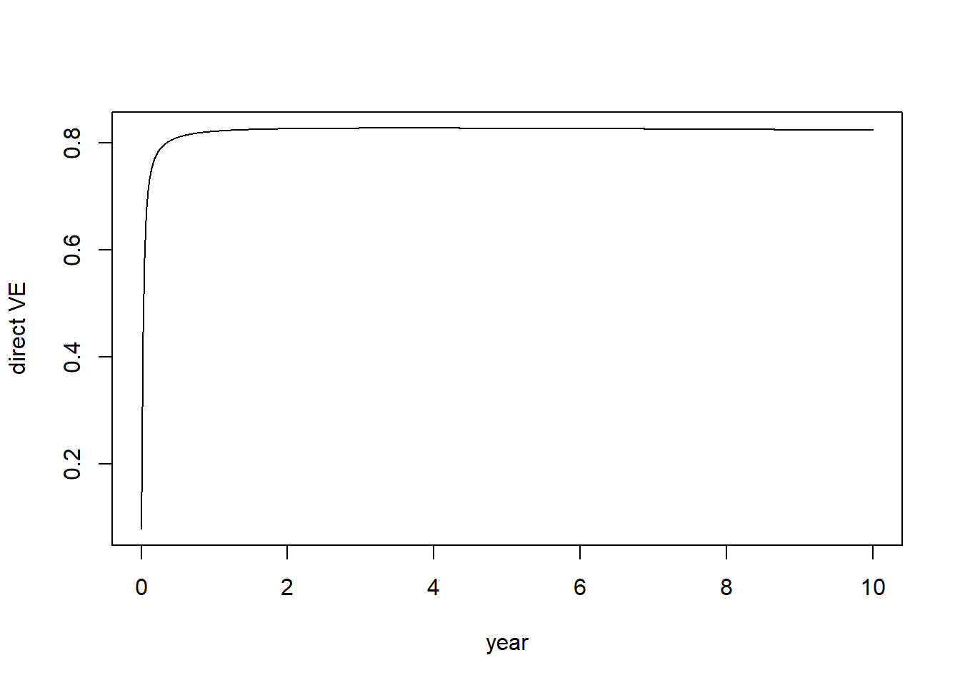
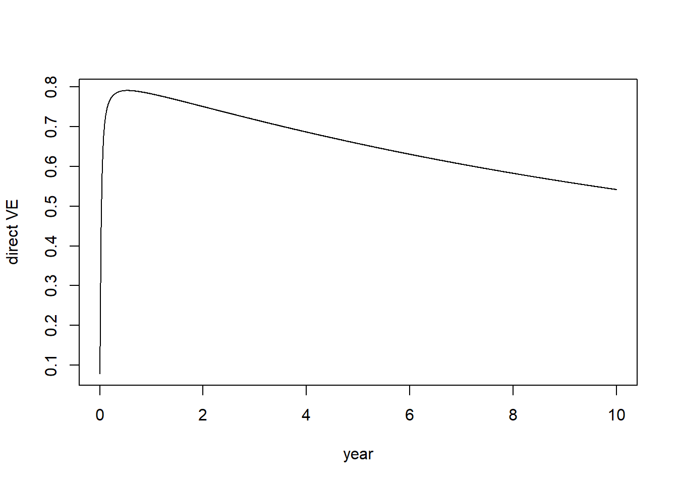
Simulation of the variable-compartment \(SEIRV\) model

Solutions for the steady states of the \(SEIR\) model. These are used to set the initial conditions as we assume that the disease transmission reached a steady state.

Ss <- "((gamma + mu) * (epsilon + mu)) / (beta * epsilon)"
Es <- "- ((gamma + mu) * (mu + omega) * ((gamma + mu) * (epsilon + mu) - beta * epsilon)) / (beta * epsilon * (gamma * (epsilon + mu + omega) + (epsilon + mu) * (mu + omega)))"

Is <- "((mu + omega) * (beta * epsilon - (gamma + mu) * (epsilon + mu))) / (beta * omega * (gamma + epsilon + mu) + beta * (gamma + mu) * (epsilon + mu))"
Rs <- "(beta * gamma * epsilon - gamma * (gamma + mu) * (epsilon + mu)) / (beta * omega * (gamma + epsilon + mu) + beta * (gamma + mu) * (epsilon + mu))"

Common parameters

R0 <- 3 # basic reproduction number
epsilon <- 1/5 # 1/epsilon = incubation period
gamma <- 1/11.8 # 1/gamma = duration of infectiousness
beta <- R0*gamma # instantaneous transmission rate
mu <- 1/(65*365) # natural death rate
omega <- 0 # re-infection is not counted in the clinical trial
omega_v <- 1/(4*365) # natural immunity waning rate
ve <- 0.834
nstg <- 1 # number of stages
N <- 1e6 # population size
f <- 1e-4 # fraction of vaccinated population
tend <- 10*365
# parameters
params <- c(nstg=nstg, epsilon=epsilon, gamma=gamma, beta=beta, 
            mu=mu, omega=omega, omega_v=omega_v, ve=ve,
            N=N, f=f, tend=tend)

# steady states for given parameters
states0 <- list(S=Ss, E=Es, I=Is, R=Rs)
steadys0 <- sapply(states0, function(x) eval(parse(text = x)))

Function to run the model

run_seirv_nstg_trial <- function(params) {
  de <- diffeqr::diffeq_setup() # to use Julia's DifferentialEquations.jl
  # initial distribution of the population across the states
  nstg <- params[["nstg"]]
  N <- params[["N"]]
  f <- params[["f"]]
  V0s <- paste(sapply(1:nstg, function(x) paste0("V", x,"=0")), collapse=",")
  eval(str2lang(paste0("u0 <- c(steadys0*N,C=0,", 
                       V0s, ",VS=0,VE=0,VI=0,VR=0,VC=0)")))
  u0[c("V1","VE","VI","VR")] <- as.numeric(steadys0*N*f/(1-f))
  tend <- params[["tend"]]
  tspan <- c(0.0, tend)
  
  prob <- de$ODEProblem(seirv_nstg_trial, u0, tspan, params)
  sol <- de$solve(prob, de$Tsit5(), saveat=1)
  mat <- sapply(sol$u, identity)
  udf <- as.data.frame(t(mat))
  out <- cbind(data.frame(t=sol$t), udf)

  Vn <- paste(sapply(1:nstg, function(x) paste0('"V', x, '"')), collapse=",")
  names(out) <- eval(str2lang(paste0('c("t","S","E","I","R","C",', Vn, 
                                     ',"VS","VE","VI","VR","VC")'))) 
  return(out)
}

Direct vaccine effectiveness in case vaccine-derived immunity does not wane over time

nstg <- params[["nstg"]]
params[["omega_v"]] <- 0
out <- run_seirv_nstg_trial(params=params)
novacc <- c("S","E","I","R")
Vn <- paste(sapply(1:nstg, function(x) paste0('"V', x, '"')), collapse=",")
vacc <- eval(str2lang(paste0('c(', Vn, ',"VS","VE","VI","VR")'))) 
  
dve <- rep(NA, nrow(out)) # direct vaccine effectiveness measured daily
for(i in 1:nrow(out)){
  dve[i] <- 1 - (out[i,"VC"]/sum(out[i,vacc]))/(out[i,"C"]/sum(out[i,novacc]))
}
plot(1:length(dve)/365, dve, type="l", ylab="direct VE", xlab="year")

Direct vaccine efficacy in case vaccine-derived immunity wanes over time with the average waiting time of 10 years

nstg <- params[["nstg"]]
params[["omega_v"]] <- 1/10/365 # average waiting time = 10 years
out <- run_seirv_nstg_trial(params=params)
novacc <- c("S","E","I","R")
Vn <- paste(sapply(1:nstg, function(x) paste0('"V', x, '"')), collapse=",")
vacc <- eval(str2lang(paste0('c(', Vn, ',"VS","VE","VI","VR")'))) 
  
dve <- rep(NA, nrow(out)) # direct vaccine effectiveness measured daily
for(i in 1:nrow(out)){
  dve[i] <- 1 - (out[i,"VC"]/sum(out[i,vacc]))/(out[i,"C"]/sum(out[i,novacc]))
}
plot(1:length(dve)/365, dve, type="l", ylab="direct VE", xlab="year")

Function to measure vaccine effectiveness over time.

measure_vacc_eff <- function(p, params, times){
  de <- diffeqr::diffeq_setup()
  params[["ve"]] <- p[1]
  params[["omega_v"]] <- p[2]
  nstg <- params[["nstg"]]
  
  out <- run_seirv_nstg_trial(params)
  novacc <- c("S","E","I","R")
  Vn <- paste(sapply(1:nstg, function(x) paste0('"V', x, '"')), collapse=",")
  vacc <- eval(str2lang(paste0('c(', Vn, ',"VS","VE","VI","VR")'))) 
  
  ve_sim <- rep(NA, length(times))
  for (i in 1:length(times)) {
    ve_sim[i] <- 1 - 
      ((out[times[i],"VC"])/sum(out[times[i],vacc])) / 
      ((out[times[i],"C"])/sum(out[times[i],novacc]))
  }
  return(ve_sim)
}

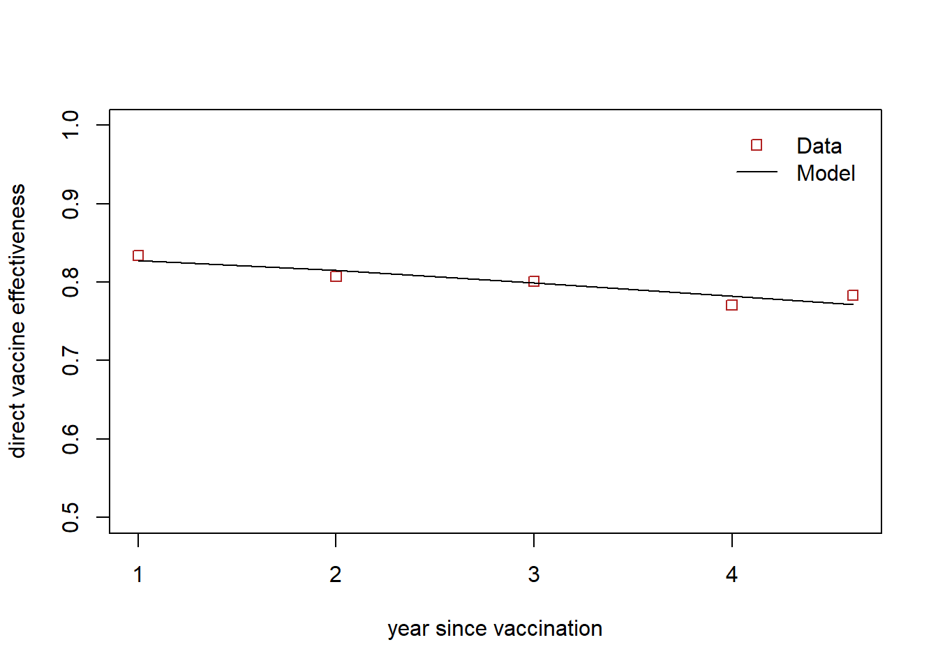
Define sum of squared difference (ssq) between the model and the data to evaluate the performance of the model.

# the initial VE is not measured from the model
times <- round(tab3[tab3$group == "Vi-TT",]$year_since_vacc*365) # times to measure VE
ve_obs <- tab3[tab3$group == "Vi-TT",]$VE_obs/100
ssq <- function(p){
  ve_sim <- measure_vacc_eff(p, params=params, times=times)
  sum((ve_obs - ve_sim)^2)  
}
# check for some predetermined ve and omega
# ssq(p=c(0.8,1/3650)) must be smaller than ssq(p=c(0.4,1/365))
ssq(p=c(0.8,1/3650))

[1] 0.05994089

ssq(p=c(0.4,1/3650))

[1] 1.005789

Estimate parameters by minimizing the ssq using the nlminb function.

params[["nstg"]] <- 1
fit1 <- nlminb(c(0.9, 1/(10*365)), objective=ssq, 
              lower=c(0.1,1/(1000*365)),
              upper=c(0.99,0.99))
fit1$par[1]

[1] 0.8589978

1/fit1$par[2]/365

[1] 22.14073

fit1$objective

[1] 0.0003437906

ve_obs

[1] 0.834 0.807 0.801 0.771 0.783

(ve_sim <- round(measure_vacc_eff(p=fit1$par, params=params, times=times), digits=3))

[1] 0.828 0.815 0.799 0.782 0.772

params[["nstg"]] <- 2
fit2 <- nlminb(c(0.9, 1/(100*365)), objective=ssq, 
              lower=c(0.1,1/(100000*365)),
              upper=c(0.99,0.99))
fit2$par[1]
1/fit2$par[2]/365
fit2$objective
ve_obs
round(measure_vacc_eff(p=fit2$par, params=params, times=times), digits=3)

Plot data and simulation results

# png("vacc_eff_obs_sim.png")
plot(times/365, ve_obs, col="firebrick", 
     ylim=c(0.5,1),  xlab="year since vaccination", ylab="direct vaccine effectiveness",
     type="p", pch=0)
lines(times/365, ve_sim, col="black")
legend("topright", 
  legend=c("Data", "Model"), 
  col=c("firebrick", "black"), 
  lty= c(0,1),
  pch=c(0,NA),
  bty = "n", 
  cex = 1.0, 
  text.col = "black", 
  horiz = F , 
  inset = c(0.02,0.02))

# dev.off()