Universal differential equation using Julia

universal differential equation

julia

sub-exponential growth

Author

Jong-Hoon Kim

Published

January 12, 2024

Universal differential equation (UDE)

The UDE refers to an approach to embed the machine learning into differential equations. The resulting UDE has some parts of the equation replaced by universal approximators i.e., neural network (NN). The UDE model approach allows us to approximate a wide, if not infinite, variety of functional relationships. As an example, I will test how well the UDE model approach will approximate a sub-exponential growth model, which is challenging to fit if we use an exponential growth model.

I am using Julia for the UDE approach as it appeared that the Julia is the most advanced in this regard.

# SciML (Scientific Machine Learning) Tools
using OrdinaryDiffEq, SciMLSensitivity
using Optimization, OptimizationOptimisers, OptimizationOptimJL

# Standard Libraries
using LinearAlgebra, Statistics

# External Libraries
using ComponentArrays, Lux, Zygote, Plots, StableRNGs
gr()

Plots.GRBackend()


# Set a random seed for reproducible behaviour
rng = StableRNG(1111)

StableRNGs.LehmerRNG(state=0x000000000000000000000000000008af)

Data generation

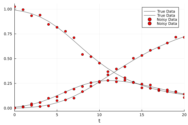
The SIR model with a sub-exponential growth is used.

function sir_subexp!(du, u, p, t)
    α, β, γ = p 
    du[1] = - β*u[1]*u[2]^α
    du[2] = + β*u[1]*u[2]^α - γ*u[2]
    du[3] = + γ*u[2]
end

sir_subexp! (generic function with 1 method)


# Define the experimental parameter
tspan = (0.0, 20.0);
# u0 = 5.0f0 * rand(rng, 2)
u0 = [0.99, 0.01, 0.0];
p_ = [0.8, 0.4, 0.2];
prob = ODEProblem(sir_subexp!, u0, tspan, p_);
solution = solve(prob, Tsit5(), abstol = 1e-12, reltol = 1e-12, saveat = 1.0);

# Add noise in terms of the mean
X = Array(solution);
t = solution.t;

xbar = mean(X, dims=2);   
noise_magnitude = 5e-2;
Xn = X .+ (noise_magnitude * xbar) .* randn(rng, eltype(X), size(X));

plot(solution, alpha = 0.75, color = :black, label = ["True Data" nothing]);
scatter!(t, transpose(Xn), color = :red, label = ["Noisy Data" nothing])

UDE model

# Let's define our Universal Differential eqution
rbf(x) = exp.(-(x .^ 2));

# Multilayer FeedForward
const U = Lux.Chain(Lux.Dense(3, 5, rbf), Lux.Dense(5, 5, rbf), 
Lux.Dense(5, 5, rbf), Lux.Dense(5, 1))

Chain(
    layer_1 = Dense(3 => 5, rbf),       # 20 parameters
    layer_2 = Dense(5 => 5, rbf),       # 30 parameters
    layer_3 = Dense(5 => 5, rbf),       # 30 parameters
    layer_4 = Dense(5 => 1),            # 6 parameters
)         # Total: 86 parameters,
          #        plus 0 states.

# Get the initial parameters and state variables of the model
p, st = Lux.setup(rng, U)

((layer_1 = (weight = Float32[-0.11597705 -0.5499123 0.10071843; -0.20088743 0.5602648 0.2718303; … ; -0.22440201 -0.57859105 0.7904316; -0.4619576 -0.62989676 0.18545352], bias = Float32[0.0; 0.0; … ; 0.0; 0.0;;]), layer_2 = (weight = Float32[-0.043933477 -0.21508422 … 0.55779475 0.5849693; 0.0011237671 0.006483868 … 0.27549765 -0.2874395; … ; 0.5079049 -0.36002874 … 0.41297784 -0.5777891; -0.5179172 -0.60432595 … -0.18625909 0.06577149], bias = Float32[0.0; 0.0; … ; 0.0; 0.0;;]), layer_3 = (weight = Float32[0.21934992 0.20916325 … -0.357856 -0.27426103; 0.59777355 -0.04514681 … 0.22668682 0.73459923; … ; 0.36797842 0.13955377 … 0.28912562 0.20840885; -0.33154675 0.035615936 … 0.011346816 -0.13401343], bias = Float32[0.0; 0.0; … ; 0.0; 0.0;;]), layer_4 = (weight = Float32[-0.49593353 -0.68478346 … -0.4632702 -0.1476636], bias = Float32[0.0;;])), (layer_1 = NamedTuple(), layer_2 = NamedTuple(), layer_3 = NamedTuple(), layer_4 = NamedTuple()))

const _st = st

(layer_1 = NamedTuple(), layer_2 = NamedTuple(), layer_3 = NamedTuple(), layer_4 = NamedTuple())


# Define the hybrid model
function ude_dynamics!(du, u, p, t, p_true)
    û = U(u, p, _st)[1] # Network prediction
    du[1] = dS = - û[1]
    du[2] = dI = + û[1] - p_true[3]*u[2] 
    du[3] = dR = + p_true[3]*u[2] 
end

ude_dynamics! (generic function with 1 method)


# Closure with the known parameter
nn_dynamics!(du, u, p, t) = ude_dynamics!(du, u, p, t, p_)

nn_dynamics! (generic function with 1 method)

# Define the problem
prob_nn = ODEProblem(nn_dynamics!, Xn[:, 1], tspan, p)

ODEProblem with uType Vector{Float64} and tType Float64. In-place: true
timespan: (0.0, 20.0)
u0: 3-element Vector{Float64}:
 1.0239505612968622
 0.0034985090690380412
 0.00031492340046744696


# I don't understand the details of the algorithm
# sensealg=QuadratureAdjoint(autojacvec=ReverseDiffVJP(true))
# I just adopted what's provided in the web page: 
# https://docs.sciml.ai/Overview/stable/showcase/missing_physics/
    
function predict(θ, X = Xn[:, 1], T = t)
    _prob = remake(prob_nn, u0 = X, tspan = (T[1], T[end]), p = θ)
    Array(solve(_prob, Tsit5(), saveat = T,
                abstol = 1e-6, reltol = 1e-6,
                sensealg=QuadratureAdjoint(autojacvec=ReverseDiffVJP(true))))
end

predict (generic function with 3 methods)


function loss(θ)
    Xhat = predict(θ)
    mean(abs2, Xn .- Xhat)
end

loss (generic function with 1 method)


losses = Float64[];

callback = function (p, l)
    push!(losses, l)
    if length(losses) % 50 == 0
        println("Current loss after $(length(losses)) iterations: $(losses[end])")
    end
    return false
end

#125 (generic function with 1 method)


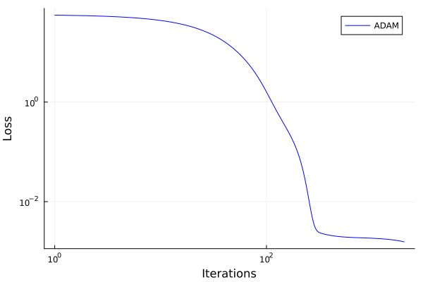
adtype = Optimization.AutoZygote();
optf = Optimization.OptimizationFunction((x, p) -> loss(x), adtype);
optprob = Optimization.OptimizationProblem(optf, ComponentVector{Float64}(p));

mxiter = 2000

res1 = Optimization.solve(optprob, ADAM(), callback = callback, maxiters = mxiter);
println("Training loss after $(length(losses)) iterations: $(losses[end])")

Training loss after 2001 iterations: 0.0015564208691683874


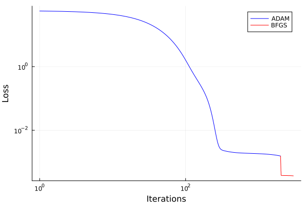
# You can optimize further by using LBFGS
optprob2 = Optimization.OptimizationProblem(optf, res1.u)

OptimizationProblem. In-place: true
u0: ComponentVector{Float64}(layer_1 = (weight = [-0.05170182389621984 -0.6044817578839353 0.030221881763510722; -0.32123561819724095 0.6510350091471692 0.44802414729182577; … ; -0.29710021515609997 -0.5198718000241755 0.8494439396600794; -0.5240838499417148 -0.5805885464625195 0.2207764494848388], bias = [0.07034258756689579; -0.1248750018606046; … ; -0.10460911230943246; -0.09231330051875483;;]), layer_2 = (weight = [-0.16444552836729504 -0.39149348409521373 … 0.4595876886836963 0.48596336484497255; 0.06110486638492416 0.09809356179876788 … 0.33257093321228715 -0.23929486432898225; … ; 0.44222617028480327 -0.07489082170130384 … 0.38613240122653225 -0.6098094519525386; -0.4255467375078114 -0.39126782596548754 … -0.07050700982314294 0.183500531584539], bias = [-0.10242371127901419; 0.05522672750843921; … ; -0.06460784045609771; 0.08515934187149939;;]), layer_3 = (weight = [0.30753421402862036 0.2947114335480522 … -0.26966507778144233 -0.19068344291102465; 0.6803575575897453 0.0350253144116066 … 0.3095389929942777 0.8122600471146871; … ; 0.4338542747333688 0.20165221719158863 … 0.35259992082403724 0.2701023387838381; -0.2070809282199827 0.1890743367589869 … 0.1659803847569096 -0.0012012794338499672], bias = [0.08539245136971987; 0.08006728472152563; … ; 0.06194248786256519; 0.15306636356417658;;]), layer_4 = (weight = [-0.42084525587118515 -0.6144846254382511 … -0.40340199958868356 -0.06553529479212013], bias = [0.09174711461704013;;]))

res2 = Optimization.solve(optprob2, Optim.LBFGS(), callback = callback, maxiters = 1000);
println("Final training loss after $(length(losses)) iterations: $(losses[end])")

Final training loss after 3002 iterations: 0.00037095070511105146


# Rename the best candidate
p_trained = res2.u

ComponentVector{Float64}(layer_1 = (weight = [0.18588559475980856 -0.678836961079842 0.003164511566198509; -0.2117593049546201 0.7659777764210745 0.5001880949174726; … ; -0.12793809908258996 -0.5806165465015546 0.7359889411458274; -0.5987978703086538 -0.8542736922318693 0.22071269547796915], bias = [0.20283880857556238; 0.1442364184846448; … ; -0.10951065483152145; -0.43136285105428973;;]), layer_2 = (weight = [-0.7722740902742339 -1.1539959612185595 … -0.2557276161227372 0.04069177034071063; 0.11613000554442242 -0.06879626497651166 … 0.49503733065196687 -0.20521706786070337; … ; 0.49449245622560034 0.17333857621023685 … 0.3021120793343474 -0.7328812254592773; -0.2225923998099525 -0.1546676318277597 … 0.38305691443718165 0.48987085385328843], bias = [-0.7211379554471269; 0.18024471356943225; … ; -0.06082478805131034; 0.35625527871182344;;]), layer_3 = (weight = [0.06379174538587522 0.13743725900849454 … -0.37275930238632443 -0.4224270345491679; 1.0145108036936996 0.5041281988482341 … 0.7904247027437314 0.9963675316648448; … ; 0.42914689744537293 0.2244122549609806 … 0.38639622079002267 0.24704090971935938; -0.2838037009222233 0.13375316701238169 … 0.12509351575197344 -0.08653639834262729], bias = [-0.1263271345517243; 0.44502442954219273; … ; 0.07338220202701212; 0.0804054739454783;;]), layer_4 = (weight = [-0.5832026087107504 -0.34311500443215825 … -0.3606462665796045 -0.2121086546094451], bias = [0.3482487547293952;;]))


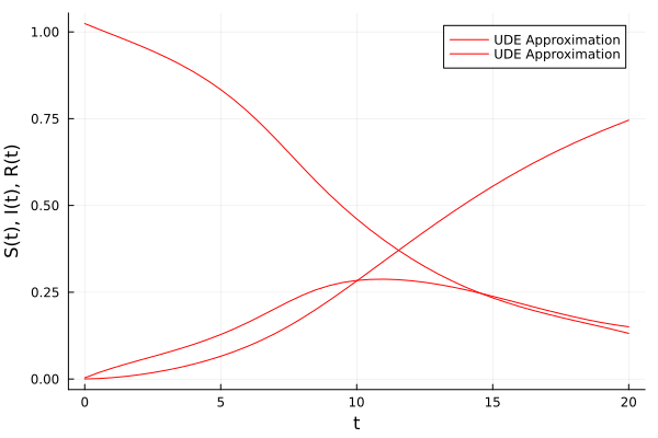
# Plot the losses
pl_losses = plot(1:mxiter, losses[1:mxiter], yaxis = :log10, xaxis = :log10,
                 xlabel = "Iterations", ylabel = "Loss", label = "ADAM", color = :blue)

plot!((mxiter+1):length(losses), losses[(mxiter+1):end], yaxis = :log10, xaxis = :log10,
      xlabel = "Iterations", ylabel = "Loss", label = "BFGS", color = :red)



## Analysis of the trained network
# Plot the data and the approximation
ts = first(solution.t):(mean(diff(solution.t)) / 2):last(solution.t)

0.0:0.5:20.0

Xhat = predict(p_trained, Xn[:, 1], ts)

3×41 Matrix{Float64}:
 1.02395      1.00815     0.992781   …  0.150512  0.141294  0.131538
 0.00349851   0.0181957   0.0310887     0.16279   0.156074  0.15051
 0.000314923  0.00141772  0.0038941     0.714463  0.730397  0.745716

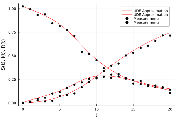
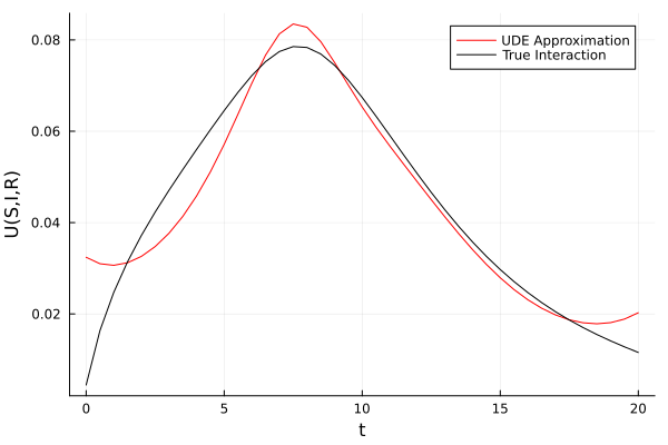
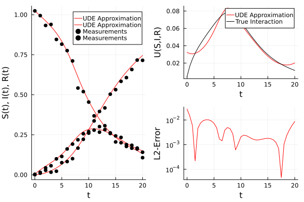
# Trained on noisy data vs real solution
pl_trajectory = plot(ts, transpose(Xhat), xlabel = "t", 
                     ylabel = "S(t), I(t), R(t)", color = :red,
                     label = ["UDE Approximation" nothing])

scatter!(solution.t, transpose(Xn), color = :black, label = ["Measurements" nothing])



# Ideal unknown interactions of the predictor
# Ybar = [-p_[2] * (Xhat[1, :] .* Xhat[2, :])'; p_[3] * (Xhat[1, :] .* Xhat[2, :])']
# Ybar = [p_[2] .* Xhat[1,:] .* (Xhat[2,:].^p_[1])]
Ybar = transpose([p_[2] * Xhat[1,i] * (Xhat[2,i].^p_[1]) for i ∈ 1:41, j ∈ 1:1])

1×41 transpose(::Matrix{Float64}) with eltype Float64:
 0.00444064  0.0163516  0.024717  …  0.0140907  0.0127893  0.0115655

# Neural network guess
Yhat = U(Xhat, p_trained, st)[1]

1×41 Matrix{Float64}:
 0.032401  0.0309925  0.0306477  0.031214  …  0.0180941  0.0188726  0.02026


pl_reconstruction = plot(ts, transpose(Yhat), xlabel = "t", 
                         ylabel = "U(S,I,R)", color = :red,
                         label = ["UDE Approximation" nothing]);

plot!(ts, transpose(Ybar), color = :black, label = ["True Interaction" nothing])



# Plot the error
pl_reconstruction_error = plot(ts, norm.(eachcol(Ybar - Yhat)), yaxis = :log, xlabel = "t",
                               ylabel = "L2-Error", label = nothing, color = :red);
pl_missing = plot(pl_reconstruction, pl_reconstruction_error, layout = (2, 1));

pl_overall = plot(pl_trajectory, pl_missing)