Estimating a time-to-event distribution in Stan

Stan instead of optim

As in the previous post, let’s create a sample through a non-homogeneous process for the infection events and a Gamma distribution for the serial (or generation) interval.

set.seed(42)
n <- 1000
tmax <- 30 # maximum time of first event
r <- 0.14 # growth rate
X <- vector("double", n)
i <- 1
ct <- 0
# generate sample through a nonhomogeneous Poisson process
while (ct < tmax) {
  t <- rexp(1, rate=exp(r*ct))
  ct <- ct + t
  X[i] <- ct
  i <- i+1
}
X <- X[X > 0]

# parameters for the serial interval
shape_true <- 2.2
scale_true <- 3.3

df <- data.frame(X=X)
si <- rgamma(length(X), shape=shape_true, scale=scale_true)
df$Y <- df$X + si

tau <- 33 # truncation time
under_tau <- df$Y < tau 
newdf <- df[under_tau,]

numerator_func <- function(x, y, parms){
  exp(r*x)*dgamma(y-x, shape=parms[[1]], scale=parms[[2]])
}

denominator_func <- function(t, parms, tmax) {
  exp(r*t)*pgamma(tmax-t, shape=parms[[1]], scale=parms[[2]])
}

# single likelihood
ll_right_trunc_exp_growth <- function(parms,x,y,tmax){
  log(numerator_func(x=x, y=y, parms=parms)) - log(integrate(denominator_func,lower=0, upper=tmax, parms=parms, tmax=tmax)$value)
}

# sum of negative log likelihoods
nll_right_trunc_exp_growth <- function(parms, X, Y, tmax){
  sll <- 0
  for(i in seq_along(X)) {
    sll <- sll + ll_right_trunc_exp_growth(parms=parms,x=X[i],y=Y[i],tmax=tmax)
  }
  return(-sll)
}

res_optim = optim(par=c(1,2), 
             fn=nll_right_trunc_exp_growth, 
             X=newdf$X, 
             Y=newdf$Y,
             tmax=tmax,
             method = "Nelder-Mead",
             control = list(maxit=2e4, reltol=1e-15))

Stan program

Gamma distribution accounting for truncation

stan_code <- "
data {
    int<lower = 0> N; // number of records
    vector<lower = 0>[N] X;
    vector<lower = 0>[N] Y;
    real tau;
}

parameters {
    real shape;
    real scale;
}

model {
    shape ~ exponential(0.1);
    scale ~ exponential(0.1);
    target += gamma_lpdf(Y - X | shape, 1/scale) - gamma_lcdf(tau-X | shape, 1/scale);
}"    

Gamma distribution accounting for truncation and exponential growth of infections

stan_code <- "
functions {
  real denominator_density(real x,
                           real xc,                
                           array[] real theta,     
                           array[] real x_r,                        
                           array[] int x_i){
    real shape = theta[1];
    real scale = theta[2];
  
    return exp(0.14 * x) * gamma_cdf(33 - x, shape, 1/scale);
  }
}
data {
    int<lower = 0> N; // number of records
    vector<lower = 0>[N] X;
    vector<lower = 0>[N] Y;
    real tau;
    real r;
}

transformed data{     
  array[0] real x_r;
  array[0] int x_i;  
} 

parameters {
    real shape;
    real scale;
}

transformed parameters {
  vector[N] log_exp_r;
  for (n in 1:N)
    log_exp_r[n] = log(exp(r*X[n]));
}

model {
    shape ~ exponential(0.1);
    scale ~ exponential(0.1);
    
    for (i in 1:N)
      target += log(exp(r*X[i])) + gamma_lpdf(Y[i] - X[i] | shape, 1/scale) -                          log(integrate_1d(denominator_density, 0, tau,
                           {shape, scale}, x_r, x_i, 1e-2));
     
}"

Compile and sample

integrate_1d(denominator_density, 0, tau, {shape, scale}, x_r, x_i, 1e-3) cause errors. Four of the two samplers generated samples if the rel_tol is increased to 1e-2 for seed=42.

library(rstan)
options(mc.cores = parallel::detectCores())
rstan_options(auto_write = TRUE)
mod <- stan_model(model_code=stan_code, verbose=TRUE)
data <- list(N=nrow(newdf), X=newdf$X, Y=newdf$Y, tau=tau, r=r)
# smp <- sampling(object=mod, data=data, seed=33, chains=4, iter=2000)
# saveRDS(smp, "stan_trunc_smp_20231124.rds")

Let’s explore the posterior distribution.

smp <- readRDS("stan_trunc_smp_20231124.rds")
df <- as.data.frame(smp)
pr <- c(0.5,0.025,0.975)
d <- as.data.frame(t(apply(df[,c("shape", "scale")],
                           2, quantile, probs=pr)))

d$name <- c("shape", "scale")
d$true <- c(shape_true, scale_true)
d$optim <- res_optim$par
d

           50%     2.5%    97.5%  name true    optim
shape 2.085903 1.760453 2.448298 shape  2.2 2.090817
scale 3.484215 2.680270 4.770225 scale  3.3 3.482427

Let’s plot the results.

library(ggplot2)
theme_set(hrbrthemes::theme_ipsum_rc(base_size=14, subtitle_size=16, axis_title_size=12))
extrafont::loadfonts()
ggplot(d)+ 
  geom_errorbar(aes(x=name, ymin=`2.5%`, ymax=`97.5%`), width=0.0)+
  geom_point(aes(x=name, y=`50%`, color="Stan"), size=3)+
  geom_point(aes(x=name, y=true, col="True value"), size=3)+
  geom_point(aes(x=name, y=optim, col="Optim"), size=3)+
  scale_color_manual(values=c("Stan"="black",
                              "True value"="firebrick", "Optim"="steelblue"))+
  labs(x="", y="", title="Median estimates with 95% CrI")+
  theme(legend.position="bottom", legend.title=element_blank())+
  scale_x_discrete(breaks=c("shape","scale"),
                   labels=c(expression(theta[1]),expression(theta[2])))+
  coord_flip()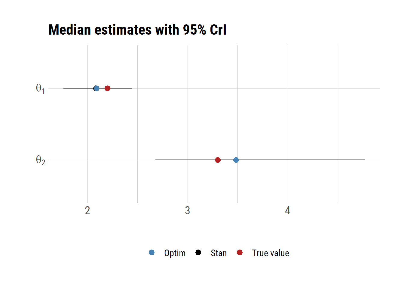

# ggsave("right_trunc_stan.png", gg, units="in", width=3.4*2, height=2.7*2)

d <- df[, c("shape","scale")]
dlong <- tidyr::pivot_longer(d, cols=c("shape","scale"),
                             names_to="param")        
dlong$param <- as.factor(dlong$param)
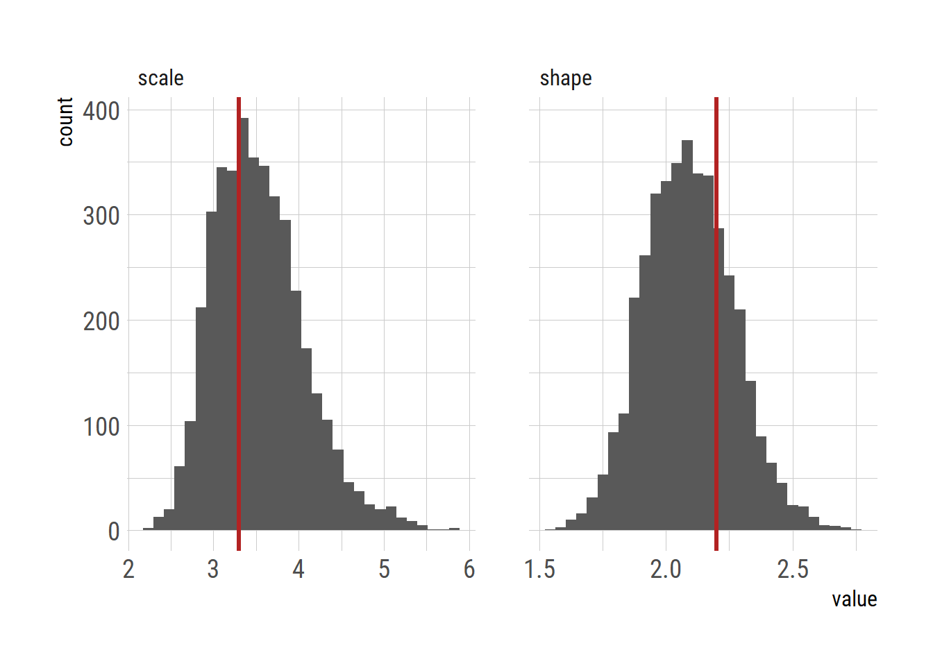
library(dplyr)
ggplot(dlong)+ 
  geom_histogram(aes(x=value))+
  facet_wrap(~param, nrow=1, scales = "free_x")+
  geom_vline(data=filter(dlong, param =="shape"), aes(xintercept=shape_true), color="firebrick", linewidth=1.2) +
  geom_vline(data=filter(dlong, param =="scale"), aes(xintercept=scale_true), color="firebrick", linewidth=1.2)