SIR model in Stan: Euler method

SIR model in Stan

I developed a SIR model and solved it an Euler method and generated a fake data as a sequence of noisy observation of daily incidence. I could have used the ODE solving routine available in Stan as in my previous post. However, an SIR model solved via the Euler method can be extended mor easily (e.g., stochatic model). I also suspect it would be easier to combine with the other statistical modeling techinques (e.g., hierarchical model), which I am going to post later.

Simulate the data

Generate \(y_{1:N}\) as a sequence of noisy observations of a daily incidence. Almost the same Stan model is used twice: once to create fake data and the second time to estimate parameters via HMC.

Stan model to create fake data

stan_code_data <- "
data {
  int<lower=0> N; // length of the data
  int<lower=0> iter_per_day;
  real dt;
  real<lower=0> S0;
  real<lower=0> I0;
  real<lower=0> R0;
  real<lower=0> CI0;
  real<lower=0> phi;
  real<lower=0> gamma;
  real<lower=0> beta;
}

parameters {

}


transformed parameters {
  vector<lower=0>[N] daily_inf;
  vector<lower=0>[N+1] S;
  vector<lower=0>[N+1] I;
  vector<lower=0>[N+1] R;
  vector<lower=0>[N+1] CI;
  
  real<lower=0> st; // susceptible at time t
  real<lower=0> it;
  real<lower=0> rt;
  real<lower=0> cit;  // cumulative infections at time t
  real<lower=0> n; // total population size
  real<lower=0> n_si; // number moving from S to I
  real<lower=0> n_ir; // number moving from I to R
  
  S[1] = S0;
  I[1] = I0;
  R[1] = R0;
  CI[1] = CI0;
    
  for (i in 2:(N+1)) {
    st = S[i-1];
    it = I[i-1];
    rt = R[i-1];
    cit = CI[i-1];
    for (j in 1:iter_per_day) {
      n = st + it + rt;
      n_si = dt * beta * st * it / n;
      n_ir = dt * gamma * it;
      st = st - n_si;
      it = it + n_si - n_ir;
      rt = rt + n_ir;
      cit = cit + n_si;
    }
    S[i] = st;
    I[i] = it;
    R[i] = rt;
    CI[i] = cit;
  }

  for (i in 2:(N+1)) {
    daily_inf[i-1] = CI[i] - CI[i-1];
  }
}

model {

}

generated quantities {
  array[N] int y_sim;
  for (i in 1:N) {
    y_sim[i] = neg_binomial_2_rng(daily_inf[i] + 1e-6, phi);
    //y_sim[i] = poisson_rng(daily_inf[i] + 1e-6);
  }
}
"

library(rstan)
options(mc.cores = parallel::detectCores())
rstan_options(auto_write = TRUE)
mod_data <- stan_model(model_code=stan_code_data, verbose=TRUE)

N=31L 
S0=999
I0=1
dt=0.1

data = list(N=N,
  S0=S0, I0=I0, R0=0, CI0=0, iter_per_day=round(1/dt),
  phi=5000, beta=0.3, gamma=0.2, dt=dt)

set.seed(42)

fit = sampling(mod_data, data=data,
                iter = 200,
                chains = 1,
                cores = 1, 
                algorithm = "Fixed_param")

df = as.data.frame(fit)
y_sim = df[, grepl("^y_sim.*", names(df))]
plot(1:N, as.numeric(y_sim[1,]))

# saveRDS(y_sim, "stan_sir_daily_inc_NB.rds")

Stan model to estimate parameters

Note that there are two parameters in the parameters block

stan_code_est <- "
data {
  int<lower=0> N;
  int<lower=0> iter_per_day;
  real dt;
  int<lower=0> y[N];
  real<lower=0> S0;
  real<lower=0> I0;
  real<lower=0> R0;
  real<lower=0> CI0;
  real<lower=0> phi;
  real<lower=0> r;
}

parameters {
  real<lower=0> gamma;
  real<lower=0> beta;
}

transformed parameters {
  vector<lower=0>[N] daily_inf;
  vector<lower=0>[N+1] S;
  vector<lower=0>[N+1] I;
  vector<lower=0>[N+1] R;
  vector<lower=0>[N+1] CI;
  
  real<lower=0> st; // susceptible at time t
  real<lower=0> it;
  real<lower=0> rt;
  real<lower=0> cit;  // cumulative infections at time t
  real<lower=0> n; // total population size
  real<lower=0> n_si; // number moving from S to I
  real<lower=0> n_ir; // number moving from I to R
  
  S[1] = S0;
  I[1] = I0;
  R[1] = R0;
  CI[1] = CI0;
    
  for (i in 2:(N+1)) {
    st = S[i-1];
    it = I[i-1];
    rt = R[i-1];
    cit = CI[i-1];
    for (j in 1:iter_per_day) {
      n = st + it + rt;
      n_si = dt * beta * st * it / n;
      n_ir = dt * gamma * it;
      st = st - n_si;
      it = it + n_si - n_ir;
      rt = rt + n_ir;
      cit = cit + n_si;
    }
    S[i] = st;
    I[i] = it;
    R[i] = rt;
    CI[i] = cit;
  }

  for (i in 2:(N+1)) {
    daily_inf[i-1] = CI[i] - CI[i-1];
  }
}


model {
  beta ~ exponential(r);
  gamma ~ exponential(r);

  y ~ neg_binomial_2(daily_inf + 1e-6, phi);

}"

library(rstan)
options(mc.cores = parallel::detectCores())
rstan_options(auto_write = TRUE)

mod_est = stan_model(model_code=stan_code_est, verbose=TRUE)

y_sim = readRDS("stan_sir_daily_inc_NB.rds")

y = as.integer(y_sim[1,])
data = list(N=length(y), y=y, S0=S0, I0=I0, R0=0, CI0=0, iter_per_day=round(1/dt), phi=50, r=0.1, dt=dt)

set.seed(42)

fit = sampling(mod_est, data=data,
                iter = 2000,
                chains = 4,
                cores = min(parallel::detectCores(), 4))

# saveRDS(fit, "stan_sir_daily_inc_NB_fit.rds")

Trace plot

library(rstan)
fit = readRDS("stan_sir_daily_inc_NB_fit.rds")
traceplot(fit, c("beta","gamma"))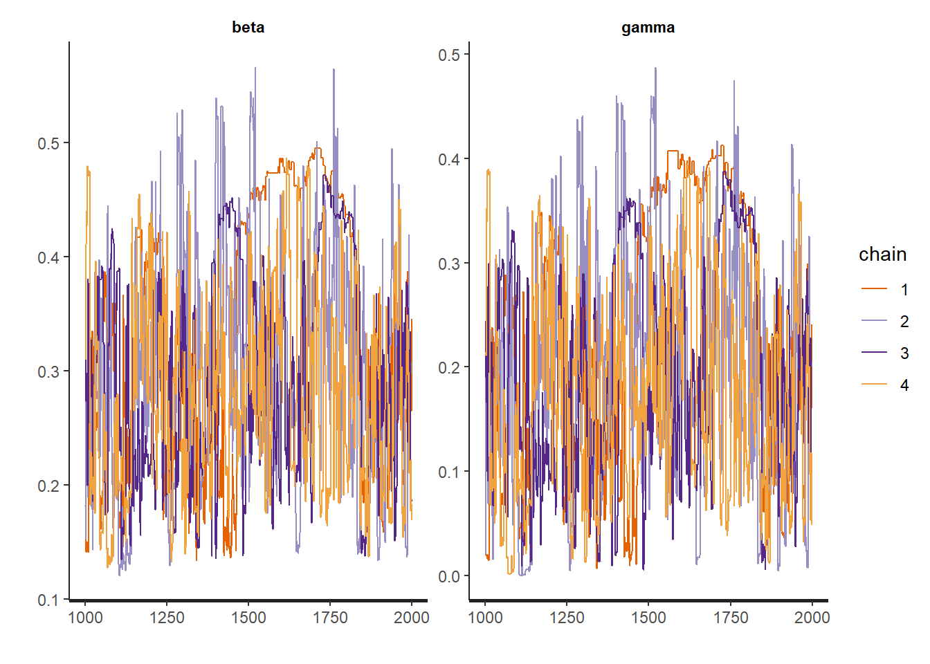

Plot the results

library(ggplot2)
extrafont::loadfonts("win", quiet=TRUE)
theme_set(hrbrthemes::theme_ipsum_rc(base_size=14, subtitle_size=16, axis_title_size=12))

df = as.data.frame(fit)
d <- df[, c("beta","gamma")]
dlong <- tidyr::pivot_longer(d, cols=c("beta","gamma"),
                             names_to="param")        
# dlong$param <- as.factor(dlong$param)
library(dplyr)
ggplot(dlong)+ 
  geom_histogram(aes(x=value))+
  facet_wrap(~param, nrow=1, scales = "free_x")+
  geom_vline(data=filter(dlong, param =="beta"), aes(xintercept=0.3), color="firebrick", linewidth=1.2) +
  geom_vline(data=filter(dlong, param =="gamma"), aes(xintercept=0.2), color="firebrick", linewidth=1.2)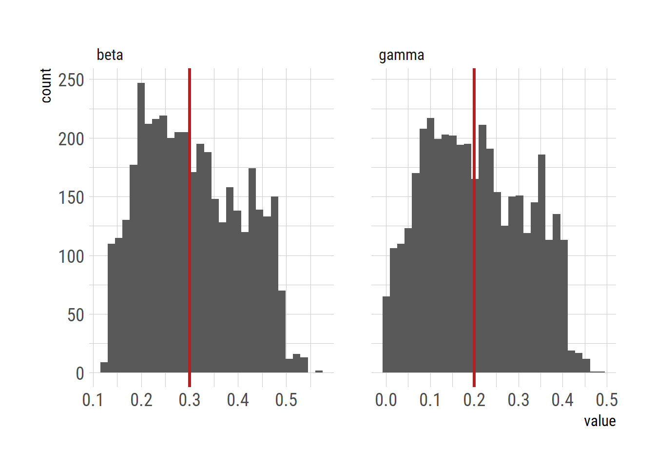

# ggsave("sir_euler_stan_param.png", gg, units="in", width=3.4*2, height=2.7*2)