Simple mathematical models with very complicated dynamics

Simple mathematical models with very complicated dynamics

Robert M. May Nature Vol. 261 June 10, 1976

This article discusses a simple first order difference equations that can display very complicated dynamics.

\[X_{t+1} = F(X_t)\]

In biological population, the nonlinear function \(F(x)\) often has the following properties. \(F(0)=0\); \(F(x)\) increases monotonically as \(X\) increases through the range of \(0<X<A\) (with \(F(x)\) attaining its maximum value at \(X=A\)); \(F(X)\) decreases monotonically as \(X\) increases beyond \(X=A\) \[N_{t+1} = N_t(a-bN_t)\]

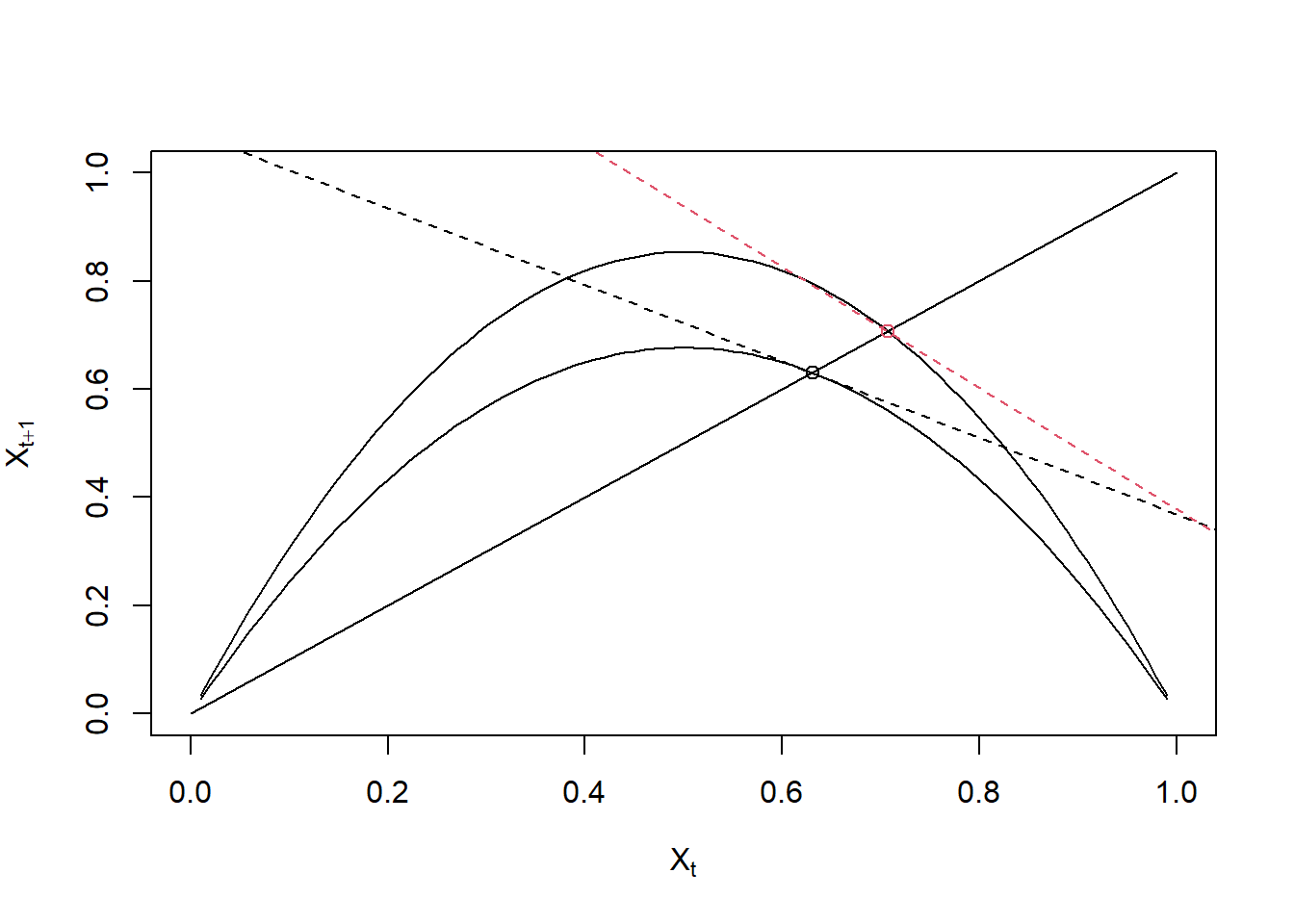
\[X_{t+1} = a X_t (1-X_t)\]

X must remain on the interval \(0<X<1\); if \(X\) ever exceeds unity, subsequent iterations diverge towards \(-\infty\). Furthermore, \(F(X)\) attains a maximum value of \(a/4\) at \(X=1/2\); the equation therefore possesses non-trivial dynamical behaviour only if \(a<4\). On the other hand, all trajectories are attracted to \(X=0\) if \(a<1\).

# function to compute the value at the next time step
# 0 < x < 1
# a < 1 for x to go to zero
# a > 4 leads to x > 1 at one point, which then leads to - infinity
# 1 < a < 4 for x to exhibit non-trivial dynamics
x_next <- function(a, x){
  a*x*(1-x)
}

x0 = seq(0.01, 0.99, 0.01)
a = c(2.707, 3.414) # values were adopted from the paper by May Nature Vol. 261 June 10, 1976
xnext = sapply(x0, function(x) x_next(a, x))

plot(x0, xnext[1,], type='l', ylim=c(0,1), xlim=c(0,1),
     xlab=expression(X[t]), ylab=expression(X[t+1]))
lines(x0, xnext[2,])
lines(0:1, 0:1) # line y = x

xstar = 1 - 1/a # points where X(t+1) = X(t)
points(xstar[1], xstar[1])
points(xstar[2], xstar[2], col=2)
# slope at the point x given a
dx <- function(a,x){
  -2*a*x+a
}

# function to compute intercept at the given slope b and point x
intcpt = function(b,x){
  x - b*x
}

abline(a=intcpt(b=dx(a=a,x=xstar[1]),x=xstar[1]), b=dx(a=a,x=xstar[1]), lty=2)
abline(a=intcpt(b=dx(a=a,x=xstar[2]),x=xstar[2]), b=dx(a=a,x=xstar[2]), lty=2, col=2)

x_iter <- function(a, x, iter, func){
  xvec = rep(NA, iter)
  xvec[1] = x
  for(i in 2:iter){
    xvec[i] = func(a, xvec[i-1])  
  }
  return(xvec)
}
plot(x_iter(2.9, 0.8, 100, x_next), type="l")

\(X_{t+1} = X_t \textrm{exp}[r(1-X_t)]\)

x_next_exp <- function(r, x){
  x*exp(r*(1-x))
}

plot(x_iter(2, 0.8, 100, x_next_exp), type="l")

x_next2 <- function(r, x){
 x1 <- a*x*(1-x)
 x2 <- a*x1*(1-x1)
 return(x2)
}

xnext = sapply(x0, function(x) x_next2(a, x))

plot(x0, xnext[1,], type='l', ylim=c(0,1), xlim=c(0,1),
     xlab=expression(X[t]), ylab=expression(X[t+2]))
lines(x0, xnext[2,])
lines(0:1, 0:1) # line y = x