Final epidemic size: uniroot vs. optimize

Final size of an epidemic

Miller 2012 shows that the final size of an epidmic for a well-mixed population can be derived in the following way. We divide the population into susceptible, infected, and recovered fractions: \(S(t), I(t), and R(t)\) respectively. Assuming a large population, constant transmission and recovery rates, and mass action mixing, we have

\[\dot{S}= -\beta IS, ~\dot{I}=\beta IS -\gamma I, ~\dot{R}=\gamma I\] We can remove \(\dot{R}\) since \(S+I+R=1\). From the equation, we can have the following relationship.

\[\frac{dS}{dI}= -1 + \frac{\gamma}{\beta S}\] Solving this equation gives the following: \[ I(t) = -S(t) + \frac{\gamma}{\beta} \text{ln} S(t) + C\]

We can find \(C=1\) using the initial conditions (\(I\rightarrow 0, S\rightarrow 0\)). Then, using \(I(\infty)=0\) gives the following relationship

\[S(\infty) = 1 − \text{exp}\left[-R_0\left(1-S(\infty)\right)\right]\] Using the \(R(\infty)=1-S(\infty)\), we can get the following equation for the final size of an epidemic, \(R(\infty)\):

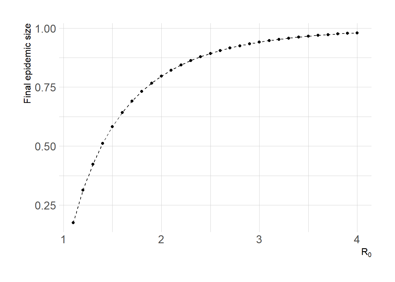
\[R(\infty) = 1 − \text{exp}\left[-R_0R(\infty)\right]\] Let’s use the above relationship to compute the final epidemic size nuerically

final_size <- function(R, R0){
  R - 1 + exp(-R0*R)
}
# lower bound set at 0.1 to avoid R=0, which is also a solution
uniroot(final_size, interval=c(0.1,1), R0=2)$root

[1] 0.796811

df <- data.frame(R0vec = c(1.1, seq(1.2, 4, by=0.1))) # as  
df$sizevec = sapply(df$R0vec, function(x) uniroot(final_size, interval=c(0.1,1), R0=x)$root)

library(ggplot2)
theme_set(hrbrthemes::theme_ipsum_rc(base_size=14, subtitle_size=16, axis_title_size=12))

ggplot(df, aes(R0vec, sizevec)) +
  geom_line(linetype="dashed")+
  geom_point()+
  labs(x=parse(text="R[0]"), y="Final epidemic size")

# ggsave("epidemicsize_R.png", p, units="in", width=3.4, height=2.7)

Instead of uniroot, optimize function can be used to find the solution for the above equation. However, optimize gives the correct answer when the function was squared.

optimize(final_size, interval=c(0.1,1), R0=2)

$minimum
[1] 0.3465758

$objective
[1] -0.1534264

final_size_sq <- function(R, R0){
  (R - 1 + exp(-R0*R))^2
}
optimize(final_size_sq, interval=c(0.1,1), R0=2)

$minimum
[1] 0.7968155

$objective
[1] 3.933157e-12