Estimating a time-to-event distribution from right-truncated data

Seamen writes: Data on time to an event are said to be right truncated if they come from a set of individuals who have been randomly sampled from a population using a sampling mechanism that selects only individuals who have experienced the event by a given time, called the truncation time.

The analysis of right-truncated data requires statistical methods that account for the fact that each of the sampled individuals must have experienced the final event by their truncation time.

Let’s assume that we are interested in estimating the serial interval and let \(X\) and \(Y\) denote the times of symptom onset of the infector and the infectee, with \(0\leq X \leq Y\). Let \(T=Y-X\) denote the serial interval. Let \(f_T^∗(t)\) and \(F_T^∗(t)\) denote, respectively, the probability density (or mass) function of \(T\) and the distribution function of \(T\). We obtain an i.i.d. sample, \((x_1, t_1), . . . , (x_n, t_n)\), from the probability distribution of \((X, T)\) given \(X + T ≤ \tau\) for some \(\tau > 0\).

\[f_{X, T}(x,t|X+T \leq \tau) = \frac{f_X(x) f^*_T(t)I(x+t \leq \tau)}{\int_0^{\tau} f_X(x') F^*_T(\tau-x')\text{d}x'}\] , where \(f_X (x)\) denotes the conditional probability density (or mass) function of \(X\) given \(X \leq \tau\), and \(I(\cdot)\) denotes the indicator function. If \(X\) and \(T\) are discrete, we shall assume, without loss of generality, that \(\tau\) is an integer. We should like to estimate \(F^∗_T(t)\)

If we assume no truncation (i.e., \(F^*_T(\tau-x)=1~ \forall x\))

During an initial period of an epidemic

Seamen provides two approaches to formulating a likelihood that can be applied during the initial period of an epidemic. The first approach is: \[f_X (x;r) = \frac{\text{exp}(rx)}{\int_0^{\tau}\text{exp}(rs)ds }=\frac{r\text{exp}(rx)}{\text{exp}(r\tau) - 1 } \propto \text{exp}(rx)\], and \(T \sim \text{Gamma}(\theta_1, \theta_2)\).

Experiment

Let’s first create samples where infectees (\(X\)) are created through a non-homogeneous Poisson process where rate, \(h\), is modeled as an exponential growth with a rate, \(r\), (i.e., \(h=\text{exp}(rt)\).

set.seed(42)
n <- 1000
tmax_i <- 30 # first events that happened only before time 30
r <- 0.14 # growth rate
X <- vector("double", n)
i <- 1
ct <- 0
# generate sample through a nonhomogeneous Poisson process
while (ct < tmax_i) {
  t <- rexp(1, rate=exp(r*ct))
  ct <- ct + t
  X[i] <- ct
  i <- i+1
}
X <- X[X > 0]

# parameters for the serial interval
shape_true <- 2.2
scale_true <- 3.3

df <- data.frame(X=X)
si <- rgamma(length(X), shape=shape_true, scale=scale_true)
df$Y <- df$X + si

tmax <- 33 # truncation time
under_tmax <- df$Y < tmax 
newdf <- df[under_tmax,]

nll <- function(parms, X, Y) -sum(dgamma(Y-X, shape=parms[[1]], scale=parms[[2]], log=TRUE))
res1 = optim(par=c(1,2), fn=nll, X=newdf$X, Y=newdf$Y,
             method = "Nelder-Mead",
            control = list(maxit=2e4, reltol=1e-15))

# 
nll_right_trunc <- function(parms, X, Y, tmax) -sum(log(dgamma(Y-X, shape=parms[[1]], scale=parms[[2]])/pgamma(tmax-X, shape=parms[[1]], scale=parms[[2]])))

# the following would not work. why?
# nll_right_trunc <- function(parms, X, Y, tmax) -sum(log(dgamma(Y-X, shape=parms[[1]], scale=parms[[2]])/pgamma(tmax, shape=parms[[1]], scale=parms[[2]])))

res2 = optim(par=c(1,2), 
             fn=nll_right_trunc, 
             X=newdf$X, 
             Y=newdf$Y,
             tmax=tmax,
             method = "Nelder-Mead",
             control = list(maxit=2e4, reltol=1e-15))

Exponential growth for \(X\)

numerator_func <- function(x, y, parms){
  exp(r*x)*dgamma(y-x, shape=parms[[1]], scale=parms[[2]])
}

# using the full probability density function
# numerator_func <- function(x, y, parms){
#   exp(r*x)/(exp(r*tmax)-1)*dgamma(y-x, shape=parms[[1]], scale=parms[[2]])
# }

# uniform distribution - same as the vanilla truncation assumption
# numerator_func <- function(x, y, parms){
#   dgamma(y-x, shape=parms[[1]], scale=parms[[2]])
# }

# NB: x is not used in this formuation but is included as params to make consistent w/ other alternative formulations
denominator_func <- function(t, x, parms, tmax) {
  exp(r*t)*pgamma(tmax-t, shape=parms[[1]], scale=parms[[2]])
}

# the following would not give the correct answer. why?
# denominator_func <- function(t, x, parms, tmax) {
#   exp(r*t)*pgamma(tmax-x-t, shape=parms[[1]], scale=parms[[2]])
# }

# same as the vanialla truncation model
# denominator_func <- function(t, x, parms, tmax) {
#   dgamma(tmax-x-t, shape=parms[[1]], scale=parms[[2]])
# }

# single likelihood
ll_right_trunc_exp_growth <- function(parms,x,y,tmax){
  log(numerator_func(x=x, y=y, parms=parms)) - log(integrate(denominator_func,lower=0, upper=tmax, x=x, parms=parms, tmax=tmax)$value)
}

# sum of negative log likelihoods
nll_right_trunc_exp_growth <- function(parms, X, Y, tmax){
  sll <- 0
  for(i in seq_along(X)) {
    sll <- sll + ll_right_trunc_exp_growth(parms=parms,x=X[i],y=Y[i],tmax=tmax)
  }
  return(-sll)
}

res3 = optim(par=c(1,2), 
             fn=nll_right_trunc_exp_growth, 
             X=newdf$X, 
             Y=newdf$Y,
             tmax=tmax,
             method = "Nelder-Mead",
             control = list(maxit=2e4, reltol=1e-15))

parmdf <- data.frame(true = c(shape_true, scale_true, shape_true*scale_true))
parmdf$no_trunc <- c(res1$par, prod(res1$par))
parmdf$trunc <- c(res2$par, prod(res2$par))
parmdf$trunc_exp_growth <- c(res3$par, prod(res3$par))

parmdf

  true no_trunc    trunc trunc_exp_growth
1 2.20 2.115872 1.932797         2.100084
2 3.30 2.273549 3.684688         3.427339
3 7.26 4.810538 7.121754         7.197701

Parameter estimates based on the methods that account for right truncation and exponential growth appear to match better with the true values than the those based on the method that accounts only for right truncation.

Plot

Let’s plot the distribution

n <- 1e5
x0 <- rgamma(n, shape=shape_true, scale=scale_true)
x1 <- rgamma(n, shape=res1$par[[1]], scale=res1$par[[2]])
x2 <- rgamma(n, shape=res2$par[[1]], scale=res2$par[[2]])
x3 <- rgamma(n, shape=res3$par[[1]], scale=res3$par[[2]])

df = data.frame(model=rep(c("True","No truncation", "Right truncated", "Right truncated, exp growth"), each=n), val=c(x0,x1,x2,x3))

library(ggplot2)
extrafont::loadfonts()
theme_set(hrbrthemes::theme_ipsum_rc(base_size=14, subtitle_size=16, axis_title_size=12))

df |> ggplot(aes(x=val, fill=model))+
  geom_density(alpha=0.2) +
  labs(x="value", y="density")+
  theme(legend.position = "bottom", 
        legend.title = element_blank())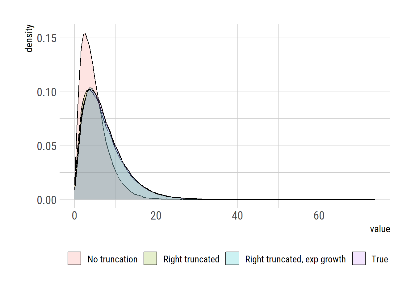

# ggsave("right_trunc2.png", gg, units="in", width=3.4*2, height=2.7*2)