Prevalence vs. incidence for the SIR model

SIR model with constant incidence rate

In the following, I implemented a simple model of disease incidence and recovery. Susceptibles are infected at a constant rate, go through the natural history of infection, and finally recover at a constant rate. Infection and recovery follow the exponential decay. This is to explore the relationship between the incidence and prevalence. 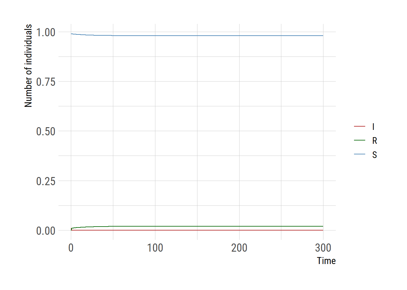If the prevalence of a disease is less than 10%, the relationship is often described as follows (e.g., see the link): \[ \text{Prevalence} = \text{IR} \times \text{Average Duration of a Disease} \] I have computed the prevalence in three ways. In particular, I assumed a short-lived infection (e.g., 2 weeks) of infectious diseases but with a long-lasting immunity. Therefore, prevalence may mean the proportion of the population immune to infection in this context. First, I use the above method. Second, I developed a simple set of differential equations to model disease incidence and recovery. Finally, I derived analytical solutions to the differential equations.

# Prevalence according to the above equation
ir <- 100/100000 # incidence rate per 100,000 person-years
dur_R <- 20 # duration of infection-derived immunity (20 years).
prev <- ir * dur_R 

# Prevalence according to the differential equation
# Note that the incidence rate (or force of infection) remains constant in this model unlike the classic SIR model.
sir_beta_const <- function(t, u, p){
  N <- sum(u)
  du1 <- - p[1]*u[1] + p[3]*u[3]
  du2 <- + p[1]*u[1] - p[2]*u[2]
  du3 <- + p[2]*u[2] - p[3]*u[3]
    
  return(list(c(du1,du2,du3))) 
}
library(deSolve)
u0 <- c(0.99, 0.01, 0)
tspan <- seq(from=0, to=300)
dur_I <- 14/365
r <- -log(1-ir) # instantaneous rate for the yearly incidence rate, ir
p <- c(r, 1/dur_I, 1/dur_R)
outdf <- as.data.frame(ode(y=u0, times=tspan, func=sir_beta_const, parms=p))

## to explore visually as well
library(ggplot2)
extrafont::loadfonts("win", quiet=TRUE)
theme_set(hrbrthemes::theme_ipsum_rc(base_size=14, subtitle_size=16, axis_title_size=12))

ggplot(outdf,aes(x=time))+
  geom_line(aes(y=`1`, color="S")) +
  geom_line(aes(y=`2`, color="I")) +
  geom_line(aes(y=`3`, color="R")) +
  scale_color_manual("",values=c("S"="steelblue","I"="firebrick",
                              "R"="darkgreen"))+
  labs(y="Number of individuals", x="Time", color="")

# Prevalence according to analytic solutions for the ODE model
# Refer to the equations below
gamma <- 1/dur_I
mu <- 0 # natural death rate, which was not implemented in the ODE model
omega <- 1/dur_R
# according the following equations
r_eq <- (r*gamma)/((gamma + mu)*(mu + omega) + r*(gamma + mu + omega))

# Compare three values
r_eq

[1] 0.01961672

tail(outdf$`3`, 1)

[1] 0.01961672

prev

[1] 0.02

The following Mathematica commands produce the steady state for S, I (written as Y below), R

# FullSimplify[Solve[{\[Mu]*(S+Y+R)-(r +\[Mu]) *S + \[Omega]* R==0, r *S-(\[Mu]+\[Gamma]) *Y == 0, \[Gamma]* Y-(\[Omega]+\[Mu])*R==0,S+Y+R==1, \[Mu]>0,r>0,\[Gamma]>0,\[Omega]>0, S>0,Y>0,R>0,S\[Element]Reals,Y\[Element]Reals,R\[Element]Reals}, {S,Y,R}]]

\[S = \frac{(\gamma +\mu ) (\mu +\omega )}{(\gamma +\mu ) (\mu +\omega )+r (\gamma +\mu +\omega )}\]

\[I =\frac{r (\mu +\omega )}{(\gamma +\mu ) (\mu +\omega )+r (\gamma +\mu +\omega )}\] \[R = \frac{\gamma r}{(\gamma +\mu ) (\mu +\omega )+r (\gamma +\mu +\omega )}\]