Particle filter using R

A simple particle filter in R

The following example was adapted from the post in RPubs.

Simulate the data

Generate \(y_{1:T}\) as a sequence of noisy observations of a latent variable \(x_{1:T}\).

# create a data set: x (latent variable) and y (observation)
set.seed(42) # to make it reproducible  (lots of random numbers follow)
T <- 50 # number of observations
x <- rep(NA, T) # latent variable
y <- rep(NA, T) # observed values
sx <- 2.2 # standard deviation for x
sy <- 0.3 # standard deviation for y
x[1] <- rnorm(1, 0, 1)
y[1] <- rnorm(1, x[1], sy)

for (t in seq(2, T)) {
  x[t] <- rnorm(1, x[t-1], sx)
  y[t] <- rnorm(1, x[t], sy)
}
x_true <- x
obs <- y

Implement a particle filter (sequential Monte Carlo)

# particle filter -----------------------------------------------------------
T <- length(y) # number of observations
N <- 100 # number of particles
# to store prior distributions for variables correspond to latent variable x
x_prior <- matrix(nrow=N, ncol = T) 
x_post <- matrix(nrow=N, ncol = T)  # posterior distributions
weights <- matrix(nrow=N, ncol = T) # weights used to draw posterior sample
W <- matrix(nrow =  N, ncol = T) # normalized weights
A <- matrix(nrow =  N, ncol = T) # indices based on the normalized weights
x_prior[, 1] <- rnorm(N, 0, sx)# initial X from a normal distribution
# calculate weights, normal likelihood
weights[, 1] <- dnorm(obs[1], x_prior[, 1], sy)
W[, 1] <- weights[, 1]/sum(weights[, 1])# normalise weights
# indices based on the weighted resampling with replacement 
A[, 1] <- sample(1:N, prob = W[1:N, 1], replace = T) 
x_post[, 1] <- x_prior[A[, 1], 1] # posterior distribution using the indices

for (t in seq(2, T)) {
  x_prior[, t] <- rnorm(N, x_post[, t-1], sx) # prior x_{t} based on x_{t-1}
  weights[, t] <- dnorm(obs[t], x_prior[, t], sy) # calculate weights 
  W[, t] <- weights[, t]/sum(weights[, t]) # normalise weights
  A[, t] <- sample(1:N, prob = W[1:N, t], replace = T) # indices
  x_post[, t] <- x_prior[A[, t], t] # posterior samples
}

Summarize results

Calculate the mean and 2.5\(^\textrm{th}\) and 97.\(^\textrm{th}\) percentile of the posterior sample as a means to get 95% credible interval.

x_means <- apply(x_post, 2, mean) # posterior mean
x_quantiles <- apply(x_post, 2, function(x) quantile(x, probs = c(0.025, 0.975))) # 95% credible interval
df <- data.frame(t = seq(1, T),
                 x_mean = x_means,
                 x_lb = x_quantiles[1, ],
                 x_ub = x_quantiles[2, ],
                 x_true = x_true, # latent variables
                 y = y) # observed values

Plot the results

library(ggplot2)
extrafont::loadfonts("win", quiet=TRUE)
theme_set(hrbrthemes::theme_ipsum_rc(base_size=14, subtitle_size=16, axis_title_size=12))
ggplot(df, aes(x = t)) +
  geom_ribbon(aes(ymin = x_lb, ymax = x_ub, fill="95% CrI"), alpha=0.5) +
  geom_line(aes(y=x_mean, color="Posterior mean")) +
  geom_line(aes(y=x_true, color="True")) +
  geom_point(aes(y=x_mean, color="Posterior mean")) +
  geom_point(aes(y=x_true, color="True")) +
  labs(y="values", x="index") + 
  scale_colour_manual("", values=c("Posterior mean"="firebrick",
                                   "True"="darkgrey")) +
  scale_fill_manual("", values="firebrick")+
  theme(legend.position = "bottom")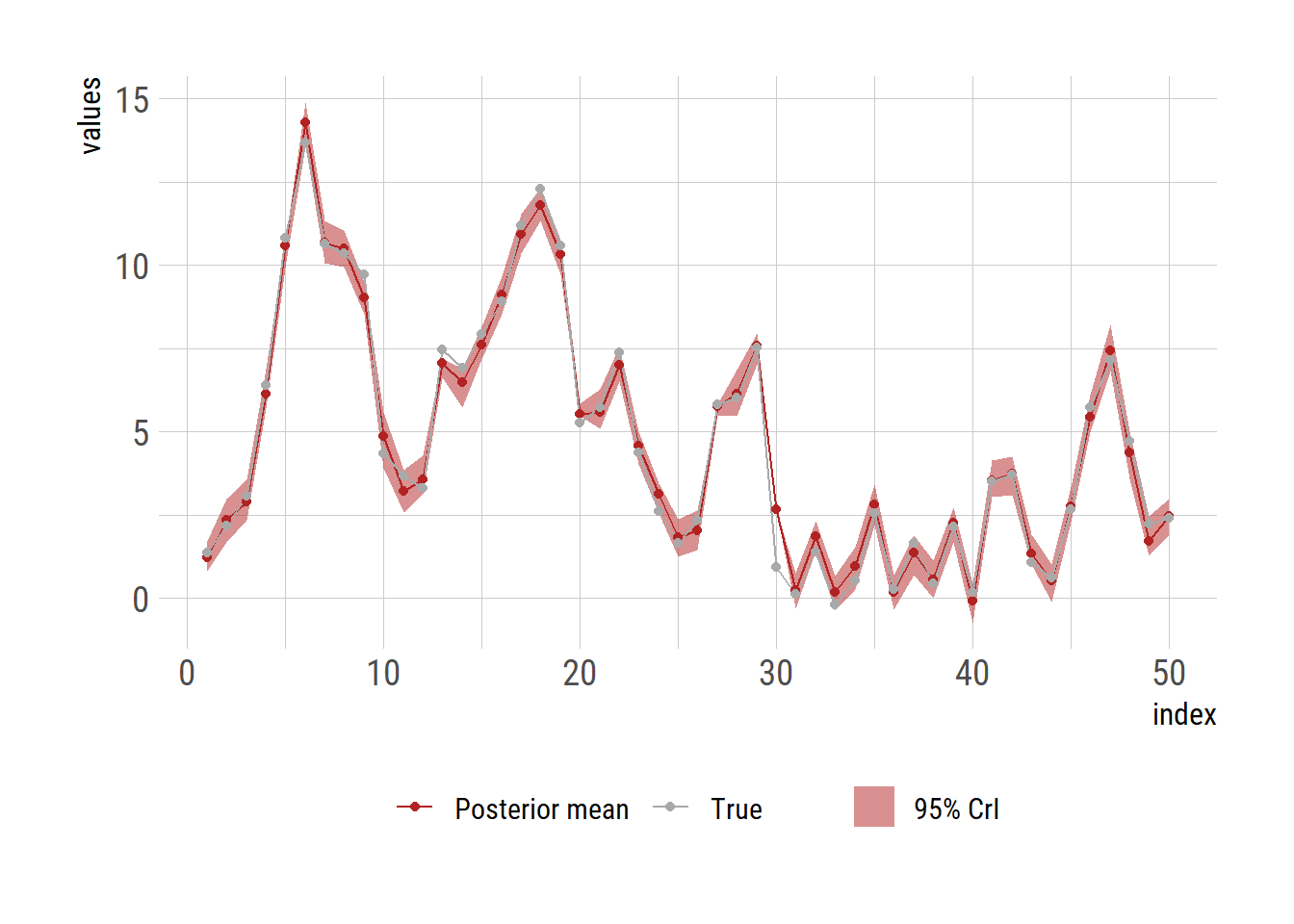

# ggsave("particle_filter.png", gg, units="in", width=3.4*2, height=2.7*2)