odin package

이번 Vaccine Impact Modeling Consoritum (VIMC) 연례회의에서 odin이라는 패키지에 대해 알게 되었다. deSolve의 업그레이드 버전이라고 보면 될까? R 코드를 C언어로 컴파일하기 때문에 최종 모형의 구동속도가 빠르다. 따라서 모형을 여러번 돌려야 하는 경우 (예를 들어 MCMC) 에 유리하다. pomp 보다도 훨씬 더 빠르다고 했는데 정확한 비교 수치는 잘 기억이 안남. 종종 C++로 모형을 만들었는데 odin 패키지를 사용하면 훨씬 쉬워질 것 같다. 좀 더 살펴보아야 할 텐데 일단 잊지 않기 위해 간단히 SIR 모형만 만들어 보았다.

Deterministic SIR model

path_sir_model <- "C:/Users/jonghoon.kim/Documents/myblog/blog/posts/odin/sir.R"
writeLines(readLines(path_sir_model))

## Core equations for transitions between compartments:
update(S) <- S - beta * S * I / N
update(I) <- I + beta * S * I / N - gamma * I
update(R) <- R + gamma * I

## Total population size (odin will recompute this at each timestep:
## automatically)
N <- S + I + R

## Initial states:
initial(S) <- S_ini # will be user-defined
initial(I) <- I_ini # will be user-defined
initial(R) <- 0

## User defined parameters - default in parentheses:
S_ini <- user(1000)
I_ini <- user(1)
beta <- user(0.2)
gamma <- user(0.1)

Run the model and plot the results

library(odin)
sir_generator <- odin::odin(path_sir_model)

x <- sir_generator$new()
# see what the object is like
# x
sir_col <- c("#8c8cd9", "#cc0044", "#999966")
x_res <- x$run(0:200)

par(mar = c(4.1, 5.1, 0.5, 0.5), las = 1)
matplot(x_res[, 1], x_res[, -1], xlab = "Time", ylab = "Number of individuals",
        type = "l", col = sir_col, lty = 1)
legend("topright", lwd = 1, col = sir_col, legend = c("S", "I", "R"), bty = "n")

Stochastic SIR model

path_sir_stoch_model <- "C:/Users/jonghoon.kim/Documents/myblog/blog/posts/odin/sir_stoch.R"
writeLines(readLines(path_sir_stoch_model))

## Core equations for transitions between compartments:
update(S) <- S - n_SI
update(I) <- I + n_SI - n_IR
update(R) <- R + n_IR

## Individual probabilities of transition:
p_SI <- 1 - exp(-beta * I / N) # S to I
p_IR <- 1 - exp(-gamma) # I to R

## Draws from binomial distributions for numbers changing between
## compartments:
n_SI <- rbinom(S, p_SI)
n_IR <- rbinom(I, p_IR)

## Total population size
N <- S + I + R

## Initial states:
initial(S) <- S_ini
initial(I) <- I_ini
initial(R) <- 0

## User defined parameters - default in parentheses:
S_ini <- user(1000)
I_ini <- user(1)
beta <- user(0.2)
gamma <- user(0.1)

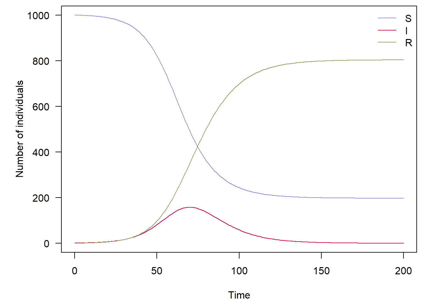
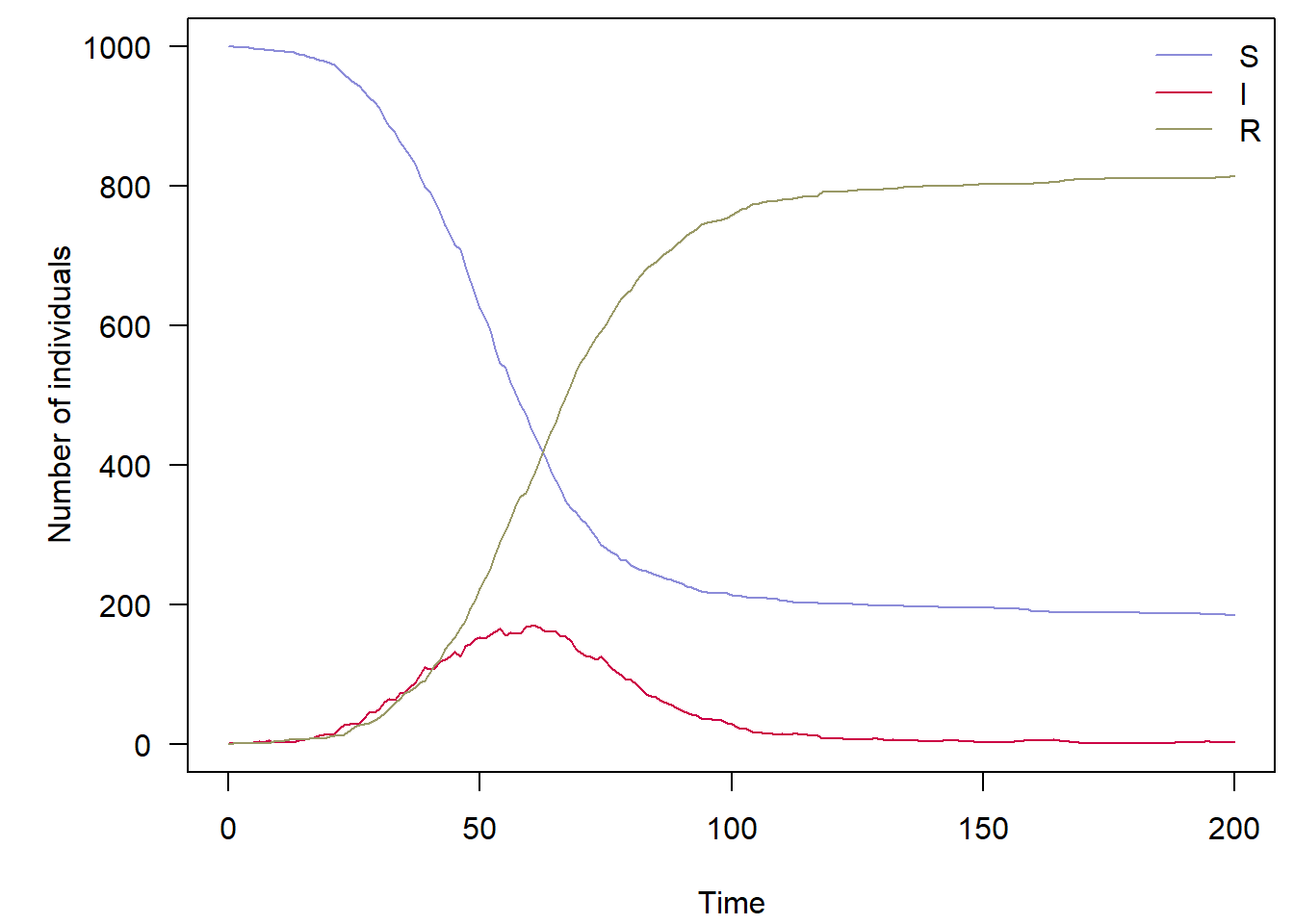
Run the model and plot the results

sir_generator <- odin::odin(path_sir_stoch_model)

set.seed(42)
x <- sir_generator$new()
x_res <- x$run(0:200)
par(mar = c(4.1, 5.1, 0.5, 0.5), las = 1)
matplot(x_res[, 1], x_res[, -1], xlab = "Time", ylab = "Number of individuals",
        type = "l", col = sir_col, lty = 1)
legend("topright", lwd = 1, col = sir_col, legend = c("S", "I", "R"), bty = "n")