ODE-based SIR models in Stan

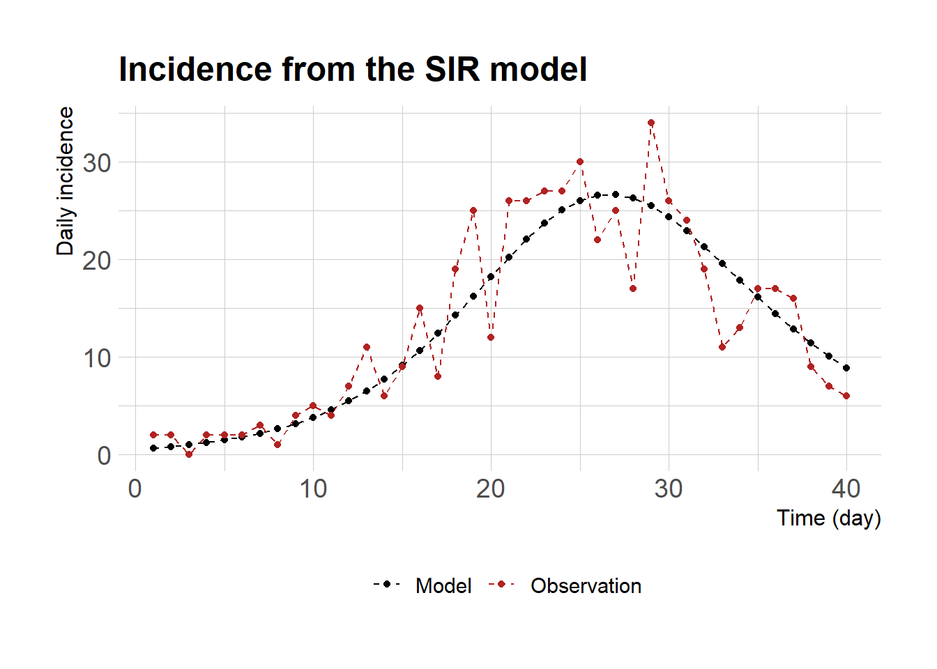
Stan은 통계 모형 뿐 아니라 ODE 모형을 시물레이션하고 모수를 추정하는 데에도 유용하다. 이 포스팅에서는 일별 감염자 자료가 주어졌을 경우 Stan을 이용하여 SIR 모형의 두 개의 모수 (\(\beta, \gamma\))를 추정하는 과정을 기술하겠다. 먼저 deSolve 패키지 양식을 따라 SIR 모형을 아래와 같이 구현하고 모형에서 예측되는 일별 감염자 자료 (dayinc) 를 평균으로 하는 거짓 관찰값을 만든다 (yobs).

sir <- function(t, state, parameters) {
  with(as.list(c(state, parameters)),{
    # rate of change
    N <- S + I + R
    dS <- - beta*S*I/N 
    dI <- + beta*S*I/N - gamma*I
    dR <- + gamma*I
    dCI <- + beta*S*I/N 
    
    # return the rate of change
    list(c(dS, dI, dR, dCI))
  }) # end with(as.list ...
}

y0 <- c(S=999, I=1, R=0, CI=0)
parms <- c(beta=0.6, gamma=0.4)
times <- seq(0, 40, by = 1)

library(dplyr)
deSolve::ode(y=y0, times=times, func=sir, parms=parms) %>% 
  as.data.frame() -> out

dayinc <- diff(out$CI)
set.seed(42)
yobs <- rpois(length(dayinc), lambda=dayinc)

df <- data.frame(time=1:length(dayinc), 
                 model=dayinc,
                 obs=yobs)
library(ggplot2)
# the ggplot theme was adopted from the following website: https://mpopov.com/tutorials/ode-stan-r/

theme_set(hrbrthemes::theme_ipsum_rc(base_size=14, subtitle_size=16, axis_title_size=12))

ggplot(df)+ 
  geom_line(aes(time, model, color="Model"), linetype="dashed")+
  geom_point(aes(time, model, color="Model"))+
  geom_line(aes(time, obs, color="Observation"), linetype="dashed")+
  geom_point(aes(time, obs, color="Observation"))+
  labs(x="Time (day)", y="Daily incidence", title="Incidence from the SIR model")+
  scale_color_manual("", values=c("Model"="black","Observation"="firebrick"))+
  theme(legend.position="bottom")

아래와 같이 Stan 모형을 만든다. Posterior predictive check 을 하기 위해 generated quantities 블록에 ypred 변수를 넣었다.

stan_code <- "functions {
  vector sir(real t,        // time
             vector y,      // state
             vector theta  // parameters
             ) {      
    vector[4] dydt;
        
    real S = y[1];
    real I = y[2];
    real R = y[3];
    real N = S + I + R;
    
    real beta = theta[1];
    real gamma = theta[2];
    
    dydt[1] = - beta * S * I / N;
    dydt[2] = beta * S * I / N - gamma * I;
    dydt[3] = gamma * I;
    dydt[4] = beta * S * I / N;
    
    return dydt;
  }
}

data {
  int<lower=1> T;
  real t0;
  array[T] real ts; 
  vector[4] y0;
  int y_obs[T];
}

parameters {
  vector<lower=0>[2] theta; // [beta, gamma]
}

model {
  array[T] vector[4] mu = ode_rk45(sir, y0, t0, ts, theta);
  real dayinc[T]; // daily incidence
  dayinc[1] = mu[1, 4] + 1e-12;
  for (t in 2:T){
    dayinc[t] = mu[t, 4] - mu[t-1, 4] + 1e-12; 
  }
  theta ~ exponential(1); // both parameters are on the positive real line
  y_obs ~ poisson(dayinc); // likelihood
}

generated quantities {
  array[T] vector[4] mu = ode_rk45(sir, y0, t0, ts, theta);
  real dayinc[T];
  dayinc[1] = mu[1, 4] + 1e-12;
  for (t in 2:T){
    dayinc[t] = mu[t,4] - mu[t-1,4] + 1e-12;
  }
  int ypred[T]; // posterior predictive 
  for (t in 1:T) {
    ypred[t] = poisson_rng(dayinc[t]);
  }
}
"

아래와 같이 Stan 모형을 이용해서 샘플링을 한다.

library(rstan)
options(mc.cores = parallel::detectCores())
rstan_options(auto_write = TRUE)

# this is for the stan model in a separate file
# mod <- stan_model(file=paste0(getwd(),"/stan/sir_stan.stan"),
#                   verbose=TRUE)
mod <- stan_model(model_code=stan_code, verbose=TRUE)
T <- 40 # end time unit for the ODE model, also the number of data points
data <- list(T=T, t0=0.0, ts=1:T, y0=c(999,1,0,0), y_obs=yobs)
smp <- sampling(object=mod, data=data, seed=42, chains=4, iter=2000)
# saveRDS(smp, "outputs/stan_smp_20230801.rds")

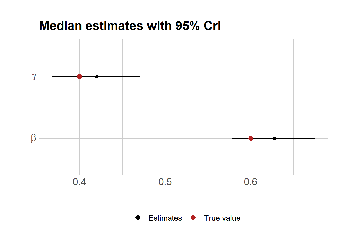
모수의 posterior 분포를 살펴보자.

# smp <- readRDS("outputs/stan_smp_20230801.rds")
smp <- readRDS("stan_smp_20230801.rds") # file is under the content/post/the_relevant_post_name/index_files/figure_html
df <- as.data.frame(smp)
pr <- c(0.5,0.025,0.975)
d <- as.data.frame(t(apply(df[,grepl("^theta.*", names(df))],
                           2, quantile, probs=pr)))
d$name <- c("beta", "gamma")
d$true <- c(0.6, 0.4)
ggplot(d)+ 
  geom_errorbar(aes(x=name, ymin=`2.5%`, ymax=`97.5%`), width=0.0)+
  geom_point(aes(x=name, y=`50%`, color="Estimates"), size=2)+
  geom_point(aes(x=name, y=true, col="True value"), size=3)+
  scale_color_manual(values=c("Estimates"="black","True value"="firebrick"))+
  labs(x="", y="", title="Median estimates with 95% CrI")+
  theme(legend.position="bottom", legend.title=element_blank())+
  scale_x_discrete(breaks=c("beta","gamma"),
                   labels=c(expression(beta),expression(gamma)))+
  coord_flip()

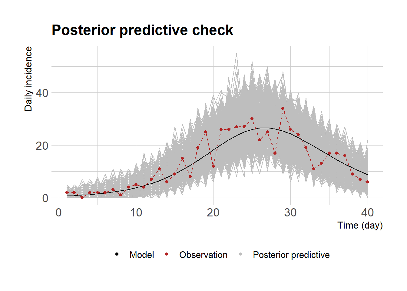
마지막으로 posterior predictive check을 통해서 모수 추정을 위해 사용했던 자료와 비교해 보자.

# pr <- c(0.5,0.025,0.975)
d <- as.data.frame(t(df[,grepl("^ypred.*", names(df))]))
d$time <- 1:40
dlong <- tidyr::pivot_longer(d, cols=-time)
dayincdf <- data.frame(inc=dayinc, time=1:40)
yobsdf <- data.frame(obs=yobs, time=1:40)

ggplot(dlong)+ 
  geom_line(aes(time, value, group=name, color="Posterior predictive"))+
  geom_line(data=dayincdf, aes(time, inc, color="Model"))+
  geom_point(data=yobsdf, aes(time, obs, color="Observation"))+
  geom_line(data=yobsdf, aes(time, obs, color="Observation"), linetype="dashed")+
  labs(x="Time (day)", y="Daily incidence", title="Posterior predictive check")+
  scale_color_manual("", values=c("Model"="black","Posterior predictive"="grey","Observation"="firebrick"))+
  theme(legend.position="bottom")