SEIR model using the Nimble pacakge

감염병 수리 모형을 개발하는 데 있어 가장 근본적인 질문 중 하나는 주어진 관찰값 (시계열)하에서 어떤 모형을 선택하고 그 모수의 값을 어떻게 결정하는가이다. 모형을 선택하는 과정은 따로 다루기로 하고 여기서는 일반적으로 사용되는 감염병 수리 모형 (i.e., SIR)을 사용할 때 모수를 추정하는 과정에 대해서 이야기해보자. 최대 가능도 (maximum likelihood) 방법에 대해서는 전에 언급하였다. 모수를 추정하는 여러 방법 중에 마르코프 연쇄 몬테카를로 (Markov Chain Monte Carlo; MCMC) 방법이 적절한 모수의 값을 찾아내고 그 값의 불확실성 (uncertainty)를 나타내는 데 가장 널리 쓰이는 방법 중의 하나이다. MCMC 알고리듬을 직접 작성해서 사용한는 것도 원리를 이해하는 데에는 도움이 되지만 이미 다양한 통계 패키지에서 MCMC가 사용되고 있으므로 기존 패키지를 사용하는 것도 합리적인 방법이 될 수 있다. 회귀 분석 등 통계모형의 경우BUGS (Bayesian Inference Using Gibbs Sampling) 혹은 JAGS (Just Another Gibbs Sampler), Stan, 그리고 NIMBLE 등에 구현된 MCMC를 사용하는 것이 많이 보편화 되어 있다.
이 중 NIMBLE 은 R 패키지 nimble을 이용해서 사용할 수 있고 패키지에서 제공하는 함수 기능을 이용해서 감염병 수리 모형을 구현하고 MCMC 까지 할 수 있다. syntax 또한 R과 유사해서 R를 사용하는 사람에게는 Stan 보다 더 접근이 용이한 것 같다. 아래에는 nimble 함수 기능을 이용하여 Euler 방법에 기반한 SIR 모형을 구현한 예이다.

library(nimble)
sir_incidence <- nimbleFunction(
  run = function(beta = double(0)) {
    tend <- 100 # 100 days of simulation
    dt <- 0.1 # time step of 0.1 day
    
    # initial condition
    St <- 999 
    It <- 1
    Rt <- 0
    CIt <- 0
    
    # create vectors for the state variables
    S <- rep(0, tend)
    I <- rep(0, tend)
    R <- rep(0, tend) 
    CI <- rep(0, tend) # cumulative incidence
    
    # first elements of the vectors are initial conditions
    S[1] <- St
    I[1] <- It
    R[1] <- Rt
    CI[1] <- CIt
  
    gamma <- 0.2 # 1/gamma = duration of infectiousness
    
    for (i in 2:tend) { # each day
      for (j in 1:ceiling(1/dt)) { # time steps per day
        Nt <- St + It + Rt                     # total population size
        rate_StoI <- St * beta * It / Nt * dt  # transition rate from S to I
        rate_ItoR <- gamma * It * dt           # transition rate from I to R
  
        dS <- - rate_StoI            # rate of change for S
        dI <- rate_StoI - rate_ItoR  # rate of change for I
        dR <- rate_ItoR              # rate of change for R
        dCI <- rate_StoI             # rate of change for cumulative incidence
      
        St <- St + dS                # update the St
        It <- It + dI                # update the It 
        Rt <- Rt + dR                # update the Rt
        CIt <- CIt + dCI             # update the CIt
      }
      S[i] <- St                     # put St in the vector 
      I[i] <- It                     # put It in the vector 
      R[i] <- Rt                     # put Rt in the vector 
      CI[i] <- CIt                   # put CIt in the vector 
   }
   # daily incidence from cumulative incidence
   inc <- CI[2:tend] - CI[1:(tend-1)] 
   return(inc) 
   returnType(double(1)) # return type
 }
)

모수 추정을 위해서 푸아송 분포를 이용하여 거짓 관찰값 (Y) 을 만들어보자.

# create observation
beta <- 0.4 # true beta
X <- sir_incidence(beta) # true daily incidence
Y <- rpois(length(X), lambda=X) # Poisson-distributed observation

아래와 같이 prior distribution, likelihood, 그리고 posterior predictive check위해서 ypred 도 함께 구현한다.

# BUGS style code
code <- nimbleCode({
  beta ~ T(dnorm(0, sd = 2), 0, 2)   # prior for beta truncated at 0 and 2
  mu[1:N] <- sir_incidence(beta)     # daily incidence from the model
  for (i in 1:N) {
    y[i] ~ dpois(mu[i])              # likelihood
    ypred[i] ~ dpois(mu[i])          # posterior predictive value
  }
})

아래와 같이 초기 조건을 설정하고 모형을 구성한다. 빠른 실행을 위해서 컴파일 한다.

# constants, data, and initial values
constants <- list(N = length(Y))      # number of observation
data <- list(y = Y)                   # observation
inits <- list(beta = 0.1)             # starting point for beta  

# create the model object
sir_model <- nimbleModel(code = code,
                         constants = constants,
                         data = data,
                         inits = inits,
                         check = FALSE)

sirMCMC <- buildMCMC(sir_model, monitors=c('beta','ypred'))
Csir <- compileNimble(sir_model)
CsirMCMC <- compileNimble(sirMCMC, project=Csir)

# thining interval was chosen based on previous analyses of ACF
samples <- runMCMC(CsirMCMC, niter=5000, thin=10, nburnin=1000)
# saveRDS(samples, "samples_nimble_20231125e.rds")

samples <- readRDS("samples_nimble_20231125e.rds")
plot(samples[,1], type="l", ylab=expression(beta), xlab="Iterations")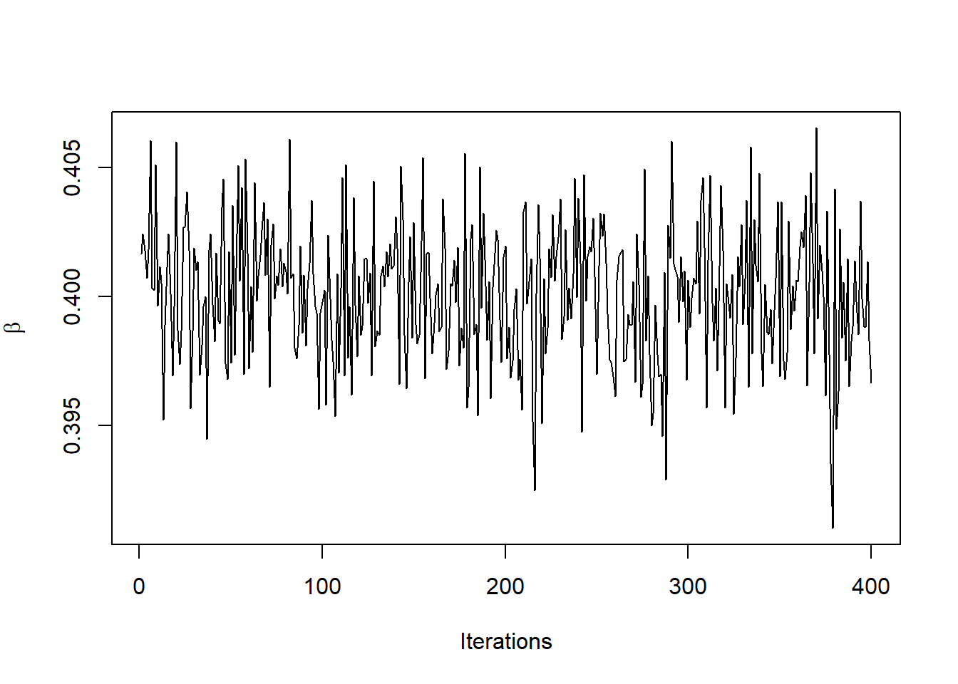

\(\beta\) 의 posterior distribution과 거짓 자료를 만들기 위해 사용했던 \(\beta\)값 (빨간색)을 비교해보자.

library(ggplot2)
extrafont::loadfonts("win", quiet=TRUE)
theme_set(hrbrthemes::theme_ipsum_rc(base_size=14, subtitle_size=16, axis_title_size=12))

samples |> 
  as.data.frame() |> 
  ggplot()+
  geom_histogram(aes(x=beta, fill="posterior"))+
  geom_vline(aes(xintercept=0.4, color="true"), linewidth=1.2)+
  labs(x=expression(beta), y="frequency")+
  scale_fill_manual("", values=c("posterior"="grey"))+
  scale_color_manual("", values=c("true"="firebrick"))+
  theme(legend.position = "bottom")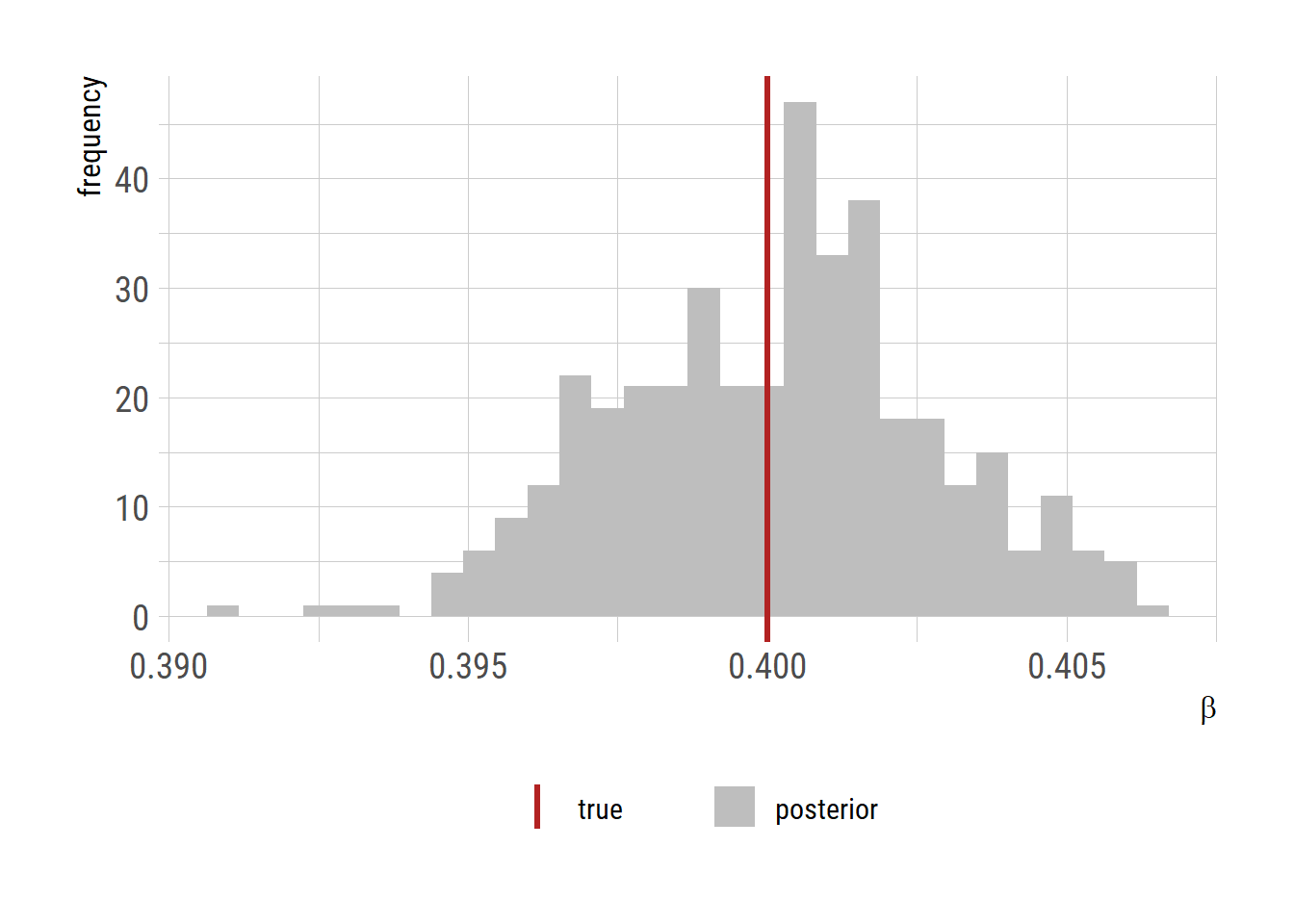

Posterior predictive check

# posterior predictive check
nsamp <- nrow(samples)
df <- data.frame(time=rep(1:99, nsamp+1), 
                 name=c(rep(1:nsamp, each=99),rep("data",99)))
df$value <- c(c(t(samples[,2:100])), Y)


library(dplyr)
ggplot(df)+
  geom_line(data=filter(df, name!="data"), aes(x=time, y=value, group=name,
            color="posterior predictive values"))+
  geom_point(data=filter(df, name=="data"), aes(x=time, y=value, color="data"),
             size=1.2) +
  labs(x='Time (day)', y='Daily infected')+
  scale_color_manual("",values=c("posterior predictive values"="grey",
                                 "data"="firebrick"))+
  theme(legend.position = "bottom")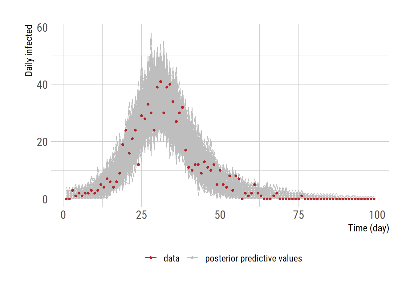

# ggsave("nimble_ppc_incidence.png", gg, units="in", width=3.4*2, height=2.7*2)