A very basic implementation of a neural network

I am documenting my learning of a neural network. The contents are mostly based on the e-book.

Load the torch library.

require(torch)

Data

# input dimensionality (number of input features)
dim_in <- 3
# number of observations in training set
n <- 200

x <- torch_randn(n, dim_in)
coefs <- c(0.2, -1.3, -0.5)
y <- x$matmul(coefs)$unsqueeze(2) + torch_randn(n, 1) # column matrix

Weights and biases

\[f(\bf{X})=\bf{XW}+b\]

Using two layers with corresponding parameters, w1, b1, w2 and b2.

\[f(\bf{X})=(\bf{XW_1}+b_1)\bf{W_2}+b_2\]

y_pred <- x$mm(w1)$add(b1)$relu()$mm(w2)$add(b2)

# dimensionality of hidden layer
dim_hidden <- 32
# output dimensionality (number of predicted features)
dim_out <- 1

# weights connecting input to hidden layer
w1 <- torch_randn(dim_in, dim_hidden, requires_grad = TRUE)
# weights connecting hidden to output layer
w2 <- torch_randn(dim_hidden, dim_out, requires_grad = TRUE)

# hidden layer bias
b1 <- torch_zeros(1, dim_hidden, requires_grad = TRUE)
# output layer bias
b2 <- torch_zeros(1, dim_out, requires_grad = TRUE)

Predicted values from the above network is computed as follows and using Rectified Linear Unit (ReLU) as the activation function

y_pred <- x$mm(w1)$add(b1)$relu()$mm(w2)$add(b2)

Then the loss function can be created as follows

loss <- (y_pred - y)$pow(2)$mean()

learning_rate <- 1e-2

### training loop ----------------------------------------

for (epoch in 1:200) {
  ### -------- Forward pass --------
  y_pred <- x$mm(w1)$add(b1)$relu()$mm(w2)$add(b2)
  
  ### -------- Compute loss -------- 
  loss <- (y_pred - y)$pow(2)$mean()
  if (epoch %% 10 == 0)
    cat("Epoch: ", epoch, "   Loss: ", loss$item(), "\n")
  
  ### -------- Backpropagation --------
  # compute gradient of loss w.r.t. all tensors with
  # requires_grad = TRUE
  loss$backward()
  
  ### -------- Update weights -------- 
  # Wrap in with_no_grad() because this is a part we don't 
  # want to record for automatic gradient computation
   with_no_grad({
     w1 <- w1$sub_(learning_rate * w1$grad)
     w2 <- w2$sub_(learning_rate * w2$grad)
     b1 <- b1$sub_(learning_rate * b1$grad)
     b2 <- b2$sub_(learning_rate * b2$grad)  
     
     # Zero gradients after every pass, as they'd
     # accumulate otherwise
     w1$grad$zero_()
     w2$grad$zero_()
     b1$grad$zero_()
     b2$grad$zero_()  
   })
}

Epoch:  10    Loss:  3.000276 
Epoch:  20    Loss:  2.144468 
Epoch:  30    Loss:  1.749418 
Epoch:  40    Loss:  1.538223 
Epoch:  50    Loss:  1.413543 
Epoch:  60    Loss:  1.33866 
Epoch:  70    Loss:  1.294799 
Epoch:  80    Loss:  1.265488 
Epoch:  90    Loss:  1.244047 
Epoch:  100    Loss:  1.226817 
Epoch:  110    Loss:  1.212944 
Epoch:  120    Loss:  1.201177 
Epoch:  130    Loss:  1.190159 
Epoch:  140    Loss:  1.178311 
Epoch:  150    Loss:  1.167546 
Epoch:  160    Loss:  1.157191 
Epoch:  170    Loss:  1.147406 
Epoch:  180    Loss:  1.13854 
Epoch:  190    Loss:  1.131134 
Epoch:  200    Loss:  1.123894 

Evaluate the model visually

# png("obs_pred.png")
y_pred <- x$mm(w1)$add(b1)$relu()$mm(w2)$add(b2)
plot(y, y_pred, xlab="Observed", ylab="Predicted", 
     main="Neural network from scratch")
abline(a=0, b=1, col="red")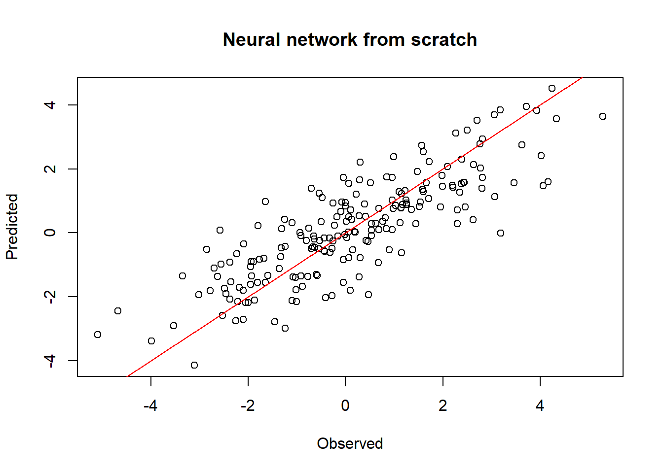

# dev.off()
sum((as.numeric(y) - as.numeric(y_pred))^2)

[1] 224.638

The same model can be created in a more compactly way using a sequential module and using the activation function.

net <- nn_sequential(
  nn_linear(dim_in, dim_hidden),
  nn_relu(),
  nn_linear(dim_hidden, dim_out)
)

Train using the Adam optimizer, a popular choice.

opt <- optim_adam(net$parameters)
# opt <- optim_sgd(net$parameters, lr=0.001)

### training loop --------------------------------------

for (epoch in 1:200) {
  # forward pass
  y_pred <- net(x)
  # compute loss 
  loss <- nnf_mse_loss(y_pred, y)
  if (epoch %% 10 == 0) { 
    cat("Epoch: ", epoch, ", Loss: ", loss$item(), "\n")
  }
  # back propagation 
  opt$zero_grad()
  loss$backward()
  # update weights
  opt$step()
}

Epoch:  10 , Loss:  3.195003 
Epoch:  20 , Loss:  2.957336 
Epoch:  30 , Loss:  2.741568 
Epoch:  40 , Loss:  2.544529 
Epoch:  50 , Loss:  2.363058 
Epoch:  60 , Loss:  2.193356 
Epoch:  70 , Loss:  2.034059 
Epoch:  80 , Loss:  1.885832 
Epoch:  90 , Loss:  1.748948 
Epoch:  100 , Loss:  1.624851 
Epoch:  110 , Loss:  1.513974 
Epoch:  120 , Loss:  1.417417 
Epoch:  130 , Loss:  1.33595 
Epoch:  140 , Loss:  1.269105 
Epoch:  150 , Loss:  1.216185 
Epoch:  160 , Loss:  1.176016 
Epoch:  170 , Loss:  1.147551 
Epoch:  180 , Loss:  1.128549 
Epoch:  190 , Loss:  1.116211 
Epoch:  200 , Loss:  1.108102 

Compare the prediction and observation

y_pred_s <- net(x)
plot(y, y_pred, xlab="Observed", ylab="Predicted", 
     main="Neural network: A sequential module")
abline(a=0, b=1, col="red")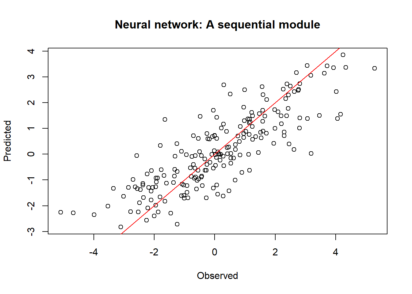

# Mean squared error, L2 loss
sum((as.numeric(y) - as.numeric(y_pred))^2)

[1] 221.6205

Compared with the linear model

xdf <- as.data.frame(as.matrix(x))
names(xdf) <- c("x1","x2", "x3")
ydf <- as.data.frame(as.matrix(y))
names(ydf) <- c("y")
dat <- cbind(xdf, ydf)
m <- lm(y~x1+x2+x3, data=dat)
y_pred_lm <- predict(m, xdf)
ydf2 <- cbind(ydf, y_pred_lm)
plot(ydf2[,1], ydf2[,2], xlab="Observed", ylab="Predicted", 
     main="Linear regresssion")
abline(a=0, b=1, col="red")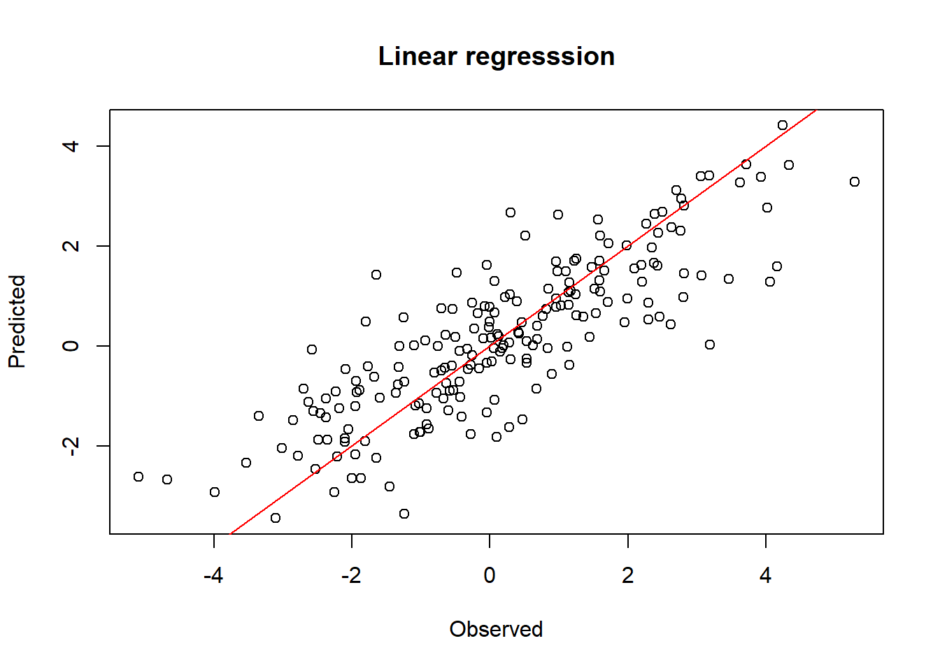

# Mean squared error, L2 loss
sum((ydf$y - y_pred_lm)^2)

[1] 218.2733