Regression using optim

Data

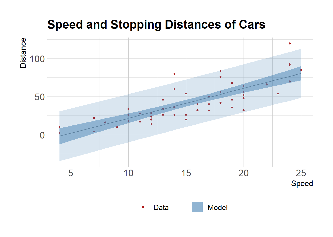
I will use the cars data with give the speed of cars and the distances taken to stop.

d <- datasets::cars
m <- lm(dist ~ speed, data=d)
summary(m)

Call:
lm(formula = dist ~ speed, data = d)

Residuals:
    Min      1Q  Median      3Q     Max 
-29.069  -9.525  -2.272   9.215  43.201 

Coefficients:
            Estimate Std. Error t value Pr(>|t|)    
(Intercept) -17.5791     6.7584  -2.601   0.0123 *  
speed         3.9324     0.4155   9.464 1.49e-12 ***
---
Signif. codes:  0 '***' 0.001 '**' 0.01 '*' 0.05 '.' 0.1 ' ' 1

Residual standard error: 15.38 on 48 degrees of freedom
Multiple R-squared:  0.6511,    Adjusted R-squared:  0.6438 
F-statistic: 89.57 on 1 and 48 DF,  p-value: 1.49e-12

Plot

Plot estimates with confidence and prediction intervals

pred <- predict(m, interval="prediction", level=0.95) # prediction interval
conf <- predict(m, interval="confidence", level=0.95) # confidence interval

mdat <- m$model
mdat$pred_estimate <- pred[,1]
mdat$pred_lb <- pred[,2]
mdat$pred_ub <- pred[,3]
mdat$conf_estimate <- conf[,1]
mdat$conf_lb <- conf[,2]
mdat$conf_ub <- conf[,3]

mdat$residuals <- residuals(m)
library(ggplot2)
library(dplyr)

theme_set(hrbrthemes::theme_ipsum_rc(base_size=14, subtitle_size=16, axis_title_size=12))

pltcar <- mdat %>% 
  ggplot(aes(speed, dist))+
  # geom_point(aes(size = abs(m$residuals)))+
  geom_point(aes(color="Data"), size = 1)+
  geom_line(aes(y=pred_estimate, color="Model"))+
  geom_ribbon(aes(ymax=pred_ub, ymin=pred_lb, fill="Model"), alpha=0.2)+
  # geom_line(aes(y=conf_estimate), color="steelblue")+
  geom_ribbon(aes(ymax=conf_ub, ymin=conf_lb, fill="Model"), alpha=0.5)+
  scale_color_manual("", values=c("Data"="firebrick"))+
  scale_fill_manual("", values=c("Model"="steelblue"))+
  labs(x="Speed", y="Distance", title="Speed and Stopping Distances of Cars")+
  theme(legend.position="bottom")

# ggsave("plot_car.png", pltcar)

pltcar

optim function

Now let’s take an alternative approach to write down the likelihood function and maximize it using the optim function

# define our likelihood function we like to optimize
negloglik <- function(par, y, X){
  sigma <- par[1]
  beta <- par[-length(par)]
  mu <- X %*% beta 
  - sum(dnorm(y, mean=mu, sd=sigma, log=TRUE), na.rm=T)
}

X = model.matrix(m)
init = c(coef(m), sigma=summary(m)$sigma)
# check
# negloglik(par=init, y=d$y, X=X)
fit <- optim(par=init, 
             fn=negloglik, 
             y=d$dist, 
             X=X, 
             control=list(reltol=1e-6))

Let’s compare the results.

fit$par

(Intercept)       speed       sigma 
 -17.579095    3.932409   15.379587 

coef(m)

(Intercept)       speed 
 -17.579095    3.932409