Learning ChatGPT 2: Approximating a tower function using a neural net

The blog post by Stephen Wolfram discusses a neural network for approximating some sort of a step function. This post is my attempt to reproduce it. A YouTube video and a book chapter by Michael Nielsen beautifully explain how a neural network can approximate a tower function while explaining the Universal Approximation Theorem.

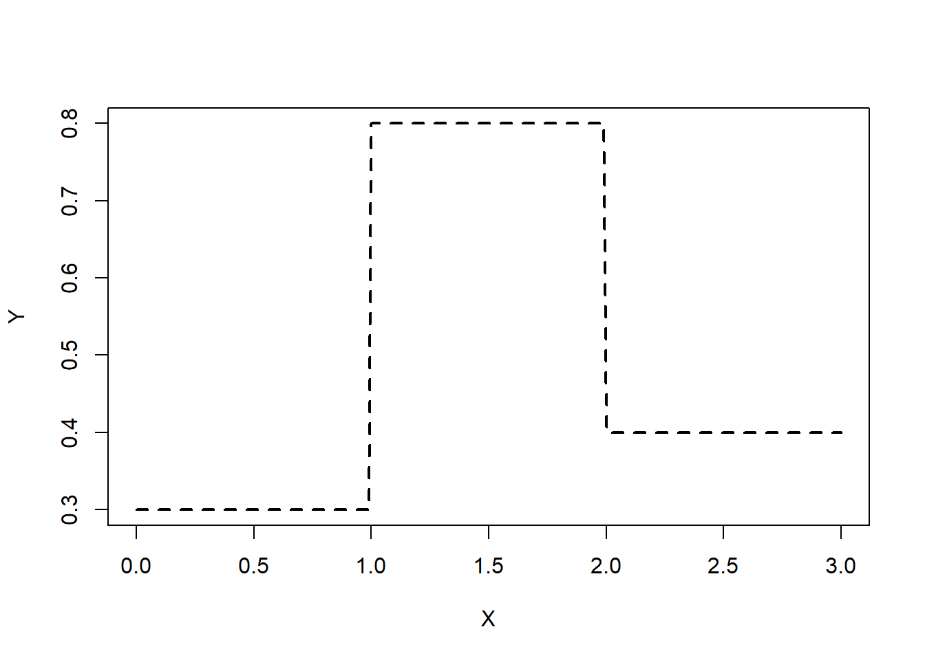
Data

library(torch)
x <- seq(0, 3,by=0.01)
y <- ifelse(x < 1, 0.3, ifelse(x < 2, 0.8, 0.4))
# input and output are turned into a 1-column tensor  
x <- torch_tensor(as.matrix(x, ncol=1))
y <- torch_tensor(as.matrix(y, ncol=1))
plot(x, y, xlab="X", type="l", ylab="Y", lty="dashed", lwd=2)

Neural network

One simple way to create a neural network is to use nn_sequential function of the torch package. Rectified linear unit (ReLU) is used for an activation function.

dim_in <- 1
dim_out <- 1
dim_hidden <- 32

net <- nn_sequential(
  nn_linear(dim_in, dim_hidden),
  nn_relu(),
  nn_linear(dim_hidden, dim_out)
)

Traing a neural network

The Adam optimizer, which a popular choice, is used.

opt <- optim_adam(net$parameters)
# opt <- optim_sgd(net$parameters, lr=0.001)

num_epochs <- 1000
for (epoch in 1:num_epochs) {
  y_pred <- net(x)  # forward pass
  loss <- nnf_mse_loss(y_pred, y)  # compute loss 
  if (epoch %% 100 == 0) { 
    cat("Epoch: ", epoch, ", Loss: ", loss$item(), "\n")
  }
  # back propagation 
  opt$zero_grad()
  loss$backward()
  opt$step()  # update weights
}

Epoch:  100 , Loss:  0.05918226 
Epoch:  200 , Loss:  0.04266065 
Epoch:  300 , Loss:  0.02848286 
Epoch:  400 , Loss:  0.01916445 
Epoch:  500 , Loss:  0.01608658 
Epoch:  600 , Loss:  0.01477717 
Epoch:  700 , Loss:  0.01393809 
Epoch:  800 , Loss:  0.01333173 
Epoch:  900 , Loss:  0.01286871 
Epoch:  1000 , Loss:  0.01249429 

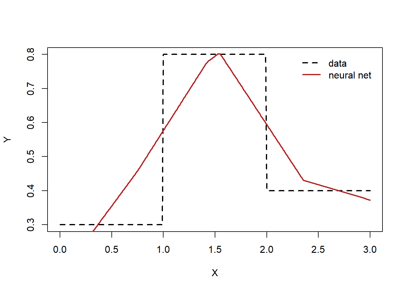
Compare the data and the model predictions

ypred <- net(x)
sprintf("L2 loss: %.4f", sum((ypred-y)^2))

[1] "L2 loss: 3.7598"

plot(x, y, type="l", xlab="X", ylab="Y", lty="dashed", lwd=2)
lines(x, ypred, lwd=2, col="firebrick")
legend("topright", 
  legend=c("data","neural net"), 
  col=c("black","firebrick"), 
  lty= c("dashed","solid"),
  lwd=2, 
  bty = "n", 
  cex = 1.0, 
  text.col = "black", 
  horiz = F , 
  inset = c(0.02,0.02))

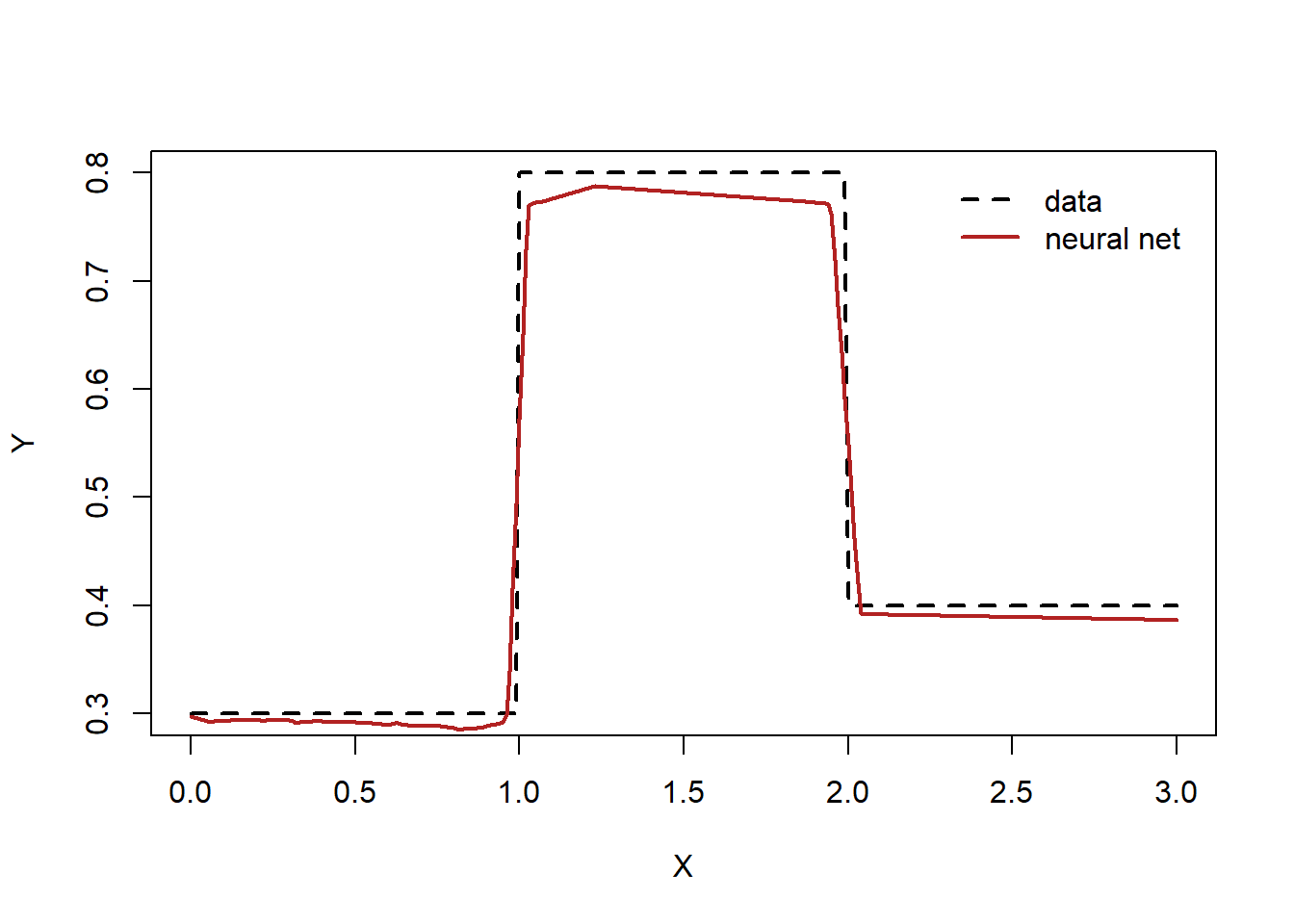
Enlarge the neural network

Let’s repeat an experiment using a larger network - more nodes and layers

dim_hidden <- 64

net <- nn_sequential(
  nn_linear(dim_in, dim_hidden),
  nn_relu(),
  nn_linear(dim_hidden, dim_hidden),
  nn_relu(),
  nn_linear(dim_hidden, dim_hidden),
  nn_relu(),
  nn_linear(dim_hidden, dim_out)
)

opt <- optim_adam(net$parameters)

num_epochs <- 1000
for (epoch in 1:num_epochs) {
  y_pred <- net(x)  # forward pass
  loss <- nnf_mse_loss(y_pred, y)  # compute loss 
  if (epoch %% 100 == 0) { 
    cat("Epoch: ", epoch, ", Loss: ", loss$item(), "\n")
  }
  # back propagation 
  opt$zero_grad()
  loss$backward()
  opt$step()  # update weights
}

Epoch:  100 , Loss:  0.02049372 
Epoch:  200 , Loss:  0.005859586 
Epoch:  300 , Loss:  0.00293437 
Epoch:  400 , Loss:  0.001943566 
Epoch:  500 , Loss:  0.001552111 
Epoch:  600 , Loss:  0.001466194 
Epoch:  700 , Loss:  0.00113698 
Epoch:  800 , Loss:  0.001119171 
Epoch:  900 , Loss:  0.0009291215 
Epoch:  1000 , Loss:  0.001042918 

Compare the data and the model predictions

ypred <- net(x)
sprintf("L2 loss: %.4f", sum((ypred-y)^2))

[1] "L2 loss: 0.3239"

# png("stepfunc_nn.png")
plot(x, y, type="l", xlab="X", ylab="Y", lty="dashed", lwd=2)
lines(x, ypred, lwd=2, col="firebrick")
legend("topright", 
  legend=c("data","neural net"), 
  col=c("black","firebrick"), 
  lty= c("dashed","solid"),
  lwd=2, 
  bty = "n", 
  cex = 1.0, 
  text.col = "black", 
  horiz = F , 
  inset = c(0.02,0.02))

# dev.off()