Kalman filter to estimate R using the FKF package

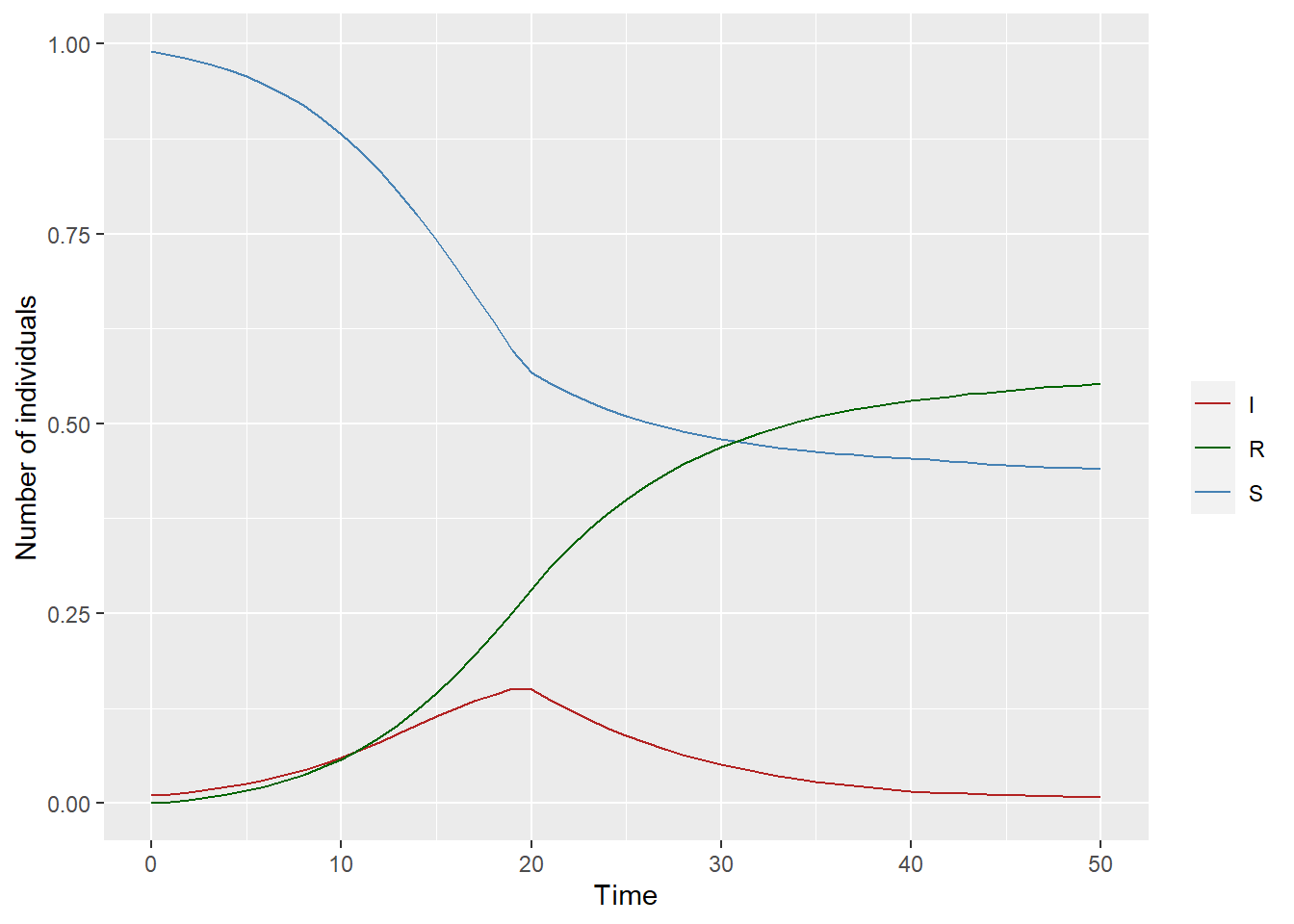
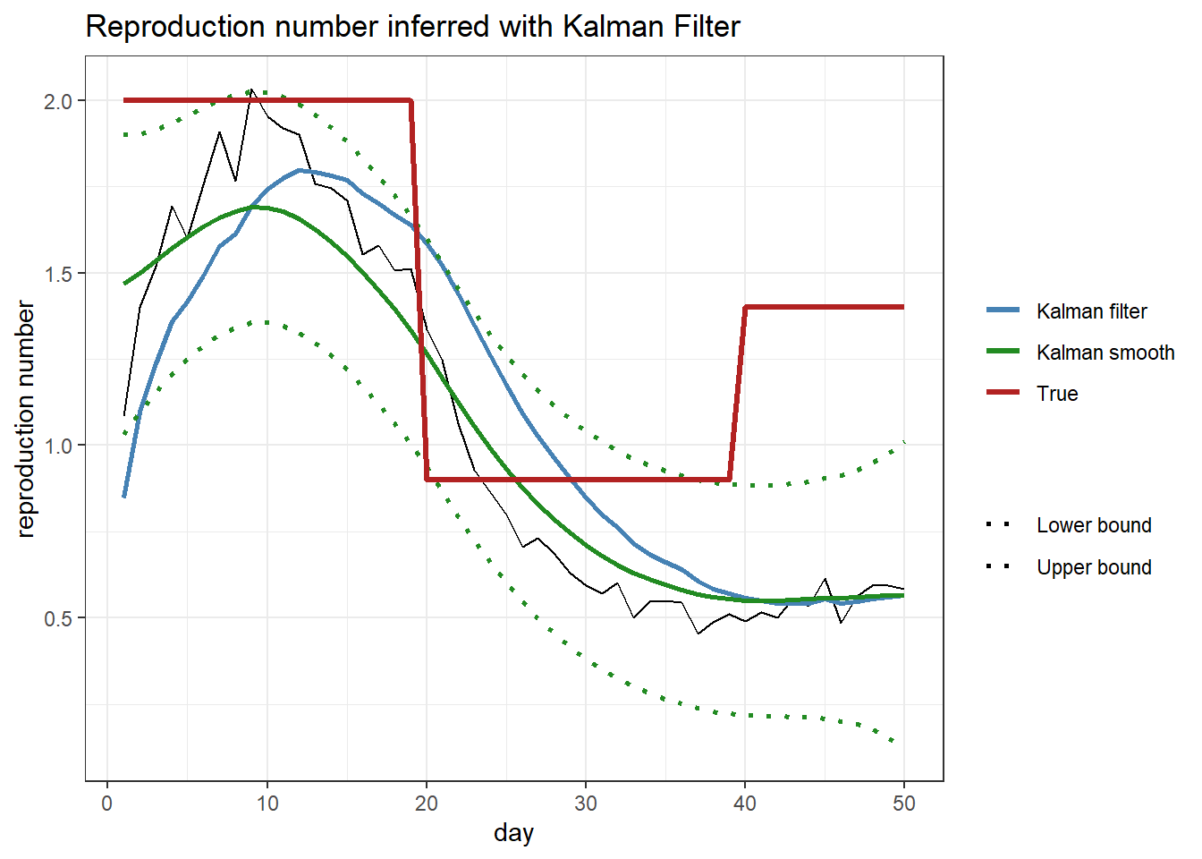
Arroyo-Marioli et al used a Kalman filter approach to estimate. I tried to reproduce in R. Let’s use a SIR model as was used in my previous post to generate growth rate time series.

library(diffeqr)
de <- diffeqr::diffeq_setup()

sir_julia <- function(u, p, t){
  N = sum(u)
  R = ifelse(t < 20, 2, ifelse(t < 40, 0.9, 1.4)) # R varies 
  p[1] = R * p[2]
  
  du1 = - p[1]*u[1]*u[2]/N
  du2 = + p[1]*u[1]*u[2]/N - p[2]*u[2]
  du3 = + p[2]*u[2]
  
  return(c(du1,du2,du3))
}

u0 <- c(0.99, 0.01, 0.0)
tspan <- c(0.0, 50.0)
p <- c(0.4, 0.2)
prob <- de$ODEProblem(sir_julia, u0, tspan, p)

# prob_jit <- diffeqr::jitoptimize_ode(de, prob)
sol <- de$solve(prob, de$Tsit5(), saveat=1)

mat <- sapply(sol$u, identity)
udf <- as.data.frame(t(mat))
tudf <- cbind(data.frame(t=sol$t), udf)

library(ggplot2)
ggplot(tudf, aes(x=t)) +
  geom_line(aes(y=V1, color="S")) +
  geom_line(aes(y=V2, color="I")) +
  geom_line(aes(y=V3, color="R")) +
  scale_color_manual("", 
                     values=c("S"="steelblue", "I"="firebrick",
                              "R"="darkgreen"))+
  labs(y="Number of individuals", x="Time", color="")

Generate daily incidence assuming 100,000 population

I <- 100000 * (tudf$V3 + 0.01) # true number of infected people at time t
case_daily <- rpois(length(I)-1, lambda=diff(I)) # observed number of infected people at t

\[I_t = (1-\gamma) I_{t-1} + \text{new cases at }t\] \[\frac{I_t-I_{t-1}}{I_{t-1}}\equiv r_t = \gamma(R_t-1) + \epsilon_i\] \[R_t = R_{t-1} + \eta_i\]

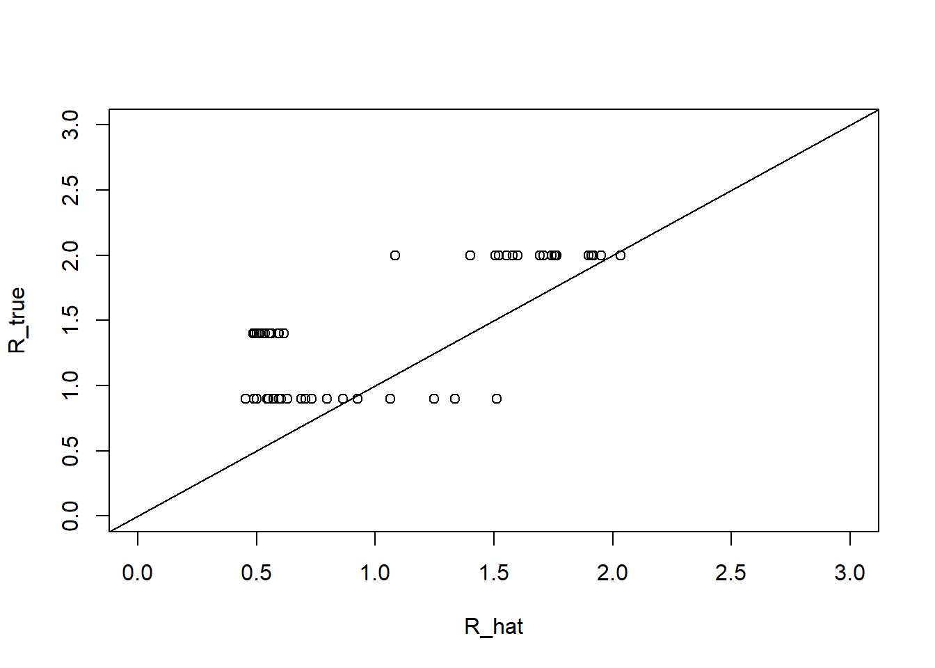
gamma <- 0.2 # recovery rate, which is the same as p[2] in the ODE model
I_hat <- rep(NA, length(case_daily)+1) # true number of infected people at time t
I_hat[1] <- I[1] # cheating, it's okay as this is the simulation check 
for (i in 2:length(I_hat)) {
  I_hat[i] <- (1-gamma)*I_hat[i-1] + case_daily[i-1]
}

It <- I_hat # observed number of infected people at t
n <- length(It)
gr <- (It[2:n] - It[1:(n-1)]) / It[1:(n-1)] # observed growth rate
t <- 1:50
R_true <- ifelse(t < 20, 2, ifelse(t < 40, 0.9, 1.4))
gr_true <- gamma * (R_true - 1)
R_hat <- gr / gamma + 1

plot(R_hat, R_true[2:(length(R_hat)+1)], xlim=c(0,3), ylim=c(0,3), 
     xlab="R_hat", ylab="R_true")
abline(a=0, b=1)

Inferring R based on the Kalman filter

library(FKF)
y <- gr
a0 <- y[1]
P0 <- matrix(1)

dt <- matrix(0)
ct <- matrix(- gamma)  
Zt <- matrix(gamma)
Tt <- matrix(1)

fit.fkf <- optim(c(HHt = var(y, na.rm = TRUE) * .5,
                   GGt = var(y, na.rm = TRUE) * .5),
                 fn = function(par, ...)
                 -fkf(HHt = matrix(par[1]), GGt = matrix(par[2]), ...)$logLik,
                 yt = rbind(y), a0 = a0, P0 = P0, dt = dt, ct = ct,
                 Zt = Zt, Tt = Tt)

# recover values
HHt <- as.numeric(fit.fkf$par[1])
GGt <- as.numeric(fit.fkf$par[2])
HHt; GGt

[1] 0.01137336

[1] -1.187671e-05

y_kf <- fkf(a0, P0, dt, ct, Tt, Zt,
             HHt = matrix(HHt), GGt = matrix(HHt),
             yt = rbind(y)) # Kalman filtering

y_ks <- fks(y_kf) # Kalman smoothing

data <- data.frame(x = seq(from = 1, to = 50, by = 1),
                   y = R_true,
                   y_hat = R_hat,
                   y_kf = as.numeric(y_kf$att),
                   y_ks = as.numeric(y_ks$ahatt),
                   y_ks_ub = as.numeric(y_ks$ahatt) + 1.96*as.numeric(sqrt(y_ks$Vt)),
                   y_ks_lb = as.numeric(y_ks$ahatt) - 1.96*as.numeric(sqrt(y_ks$Vt)))

ggplot(data, aes(x = x)) +
  geom_line(aes(y = y_hat)) +
  geom_line(aes(y = y_kf, color = "Kalman filter"), linewidth=1) +
  geom_line(aes(y = y_ks, color = "Kalman smooth"), linewidth=1) +
  geom_line(aes(y = y_ks_ub, color = "Kalman smooth", linetype="Upper bound"), linewidth=1) +
  geom_line(aes(y = y_ks_lb, color = "Kalman smooth", linetype="Lower bound"), linewidth=1) +
  geom_line(aes(y = y, color = "True"), linewidth=1.2) +
  xlab("day") + ylab("reproduction number") +
  ggtitle("Reproduction number inferred with Kalman Filter") +
  theme_bw()+
  scale_color_manual("", values=c("True"="firebrick","Kalman filter"="steelblue",
                                  "Kalman smooth"="forestgreen"))+
  scale_linetype_manual("", values=c("Upper bound"="dotted",
                                     "Lower bound"="dotted"))