LabelledArrays and NamedTupleTools make it easy to use the ODE model in Julia

SEIR model using LabelledArrays

The LabelledArrays package makes it easy to use the ODE model in Julia. It offers a method to manage variables via keys instead of indices. Variables can be constructed using the @LArray macro or LVector.

However, using arrays to store a mix of information types is not optimal for performance. I frequently need to store different variable types within a single parameter, which prompts a warning, highlighting that combining variable types in an array could reduce performance and suggesting tuples as a more efficient alternative.

┌ Warning: Utilizing arrays or dictionaries to store parameters of diverse types can compromise performance. │ Using tuples is advised for better efficiency. └ @ SciMLBase C:.kim.julia_warnings.jl:32

Tuples, being essentially immutable, presents a challenge since some of model parameters that must be adjustible or estimated. The NamedTupleTools package offers a convenient solution with its merge function, enabling easy updates to the values within a Tuple.

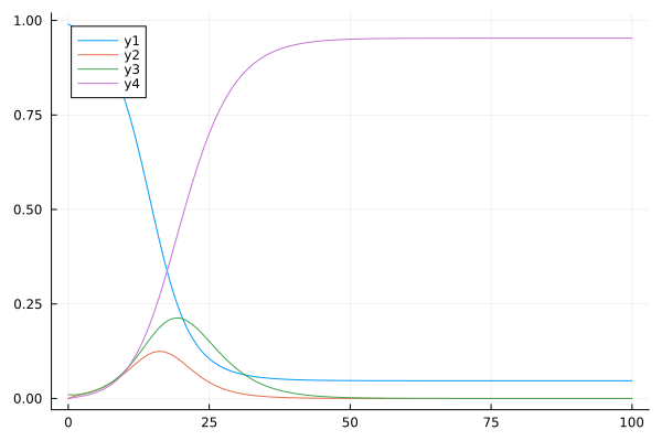
In conclusion, the best approach seems to be leveraging LabelledArrays for state variables and NamedTupleTools for parameters. Let’s delve into this approach using the SEIR model as a case study.

using LabelledArrays, OrdinaryDiffEq, Plots, NamedTupleTools, BenchmarkTools

function seir(du, u, p, t)
    N = sum(u)
    du.S = - p.β * u.S * u.I / N
    du.E = + p.β * u.S * u.I / N - p.ϵ * u.E
    du.I = + p.ϵ * u.E - p.γ* u.I
    du.R = + p.γ* u.I 
end

seir (generic function with 1 method)

u0 = @LArray [0.99, 0.0, 0.01, 0.0] (:S, :E, :I, :R);
p_la = @LArray [0.5, 1/2, 1/4] (:β, :ϵ, :γ);
p_la = LVector(p_la, β=0.8, str="string", int=9, la=LVector(a=1,b=2,c=3), tp=(a=1,b=2,c=3));
tspan = (0.0, 100.0);
prob = ODEProblem(seir, u0, tspan, p_la);
sol = solve(prob, Tsit5(), saveat=1);

s = [sol[i].S for i in 1:101];
e = [sol[i].E for i in 1:101];
i = [sol[i].I for i in 1:101];
r = [sol[i].R for i in 1:101];

plot(sol.t, [s e i r])

# NamedTupleTools approach
p_nt = (β=0.5, ϵ=1/2, γ=1/4);
p_nt = merge(p_nt, (β=0.8, str="string", int=9, la=LVector(a=1,b=2,c=3), tp=(a=1,b=2,c=3)));

using BenchmarkTools
time_la = @benchmark solve(ODEProblem(seir, u0, tspan, p_la), Tsit5(), saveat=1);
time_nt = @benchmark solve(ODEProblem(seir, u0, tspan, p_nt), Tsit5(), saveat=1);
time_la

BenchmarkTools.Trial: 10000 samples with 1 evaluation.
 Range (min … max):  180.800 μs … 345.339 ms  ┊ GC (min … max): 0.00% … 99.84%
 Time  (median):     234.550 μs               ┊ GC (median):    0.00%
 Time  (mean ± σ):   400.856 μs ±   3.459 ms  ┊ GC (mean ± σ):  9.26% ±  3.45%

  █▅▃▃▂▂▁ ▄▁ ▄▃▁ ▃▂▄▃▃▃▂▂▁▁▁▁▁                                  ▁
  █████████████████████████████████▇▇▇▇▆▆▅▆▅▅▃▅▅▅▅▅▄▅▅▅▄▅▅▅▄▅▅▅ █
  181 μs        Histogram: log(frequency) by time       1.35 ms <

 Memory estimate: 107.62 KiB, allocs estimate: 5775.

time_nt

BenchmarkTools.Trial: 10000 samples with 1 evaluation.
 Range (min … max):   59.800 μs … 273.123 ms  ┊ GC (min … max):  0.00% … 99.92%
 Time  (median):      91.100 μs               ┊ GC (median):     0.00%
 Time  (mean ± σ):   161.812 μs ±   2.731 ms  ┊ GC (mean ± σ):  16.86% ±  1.00%

  █▇▆▆▆▄▂▁▂▂ ▃▅▆▄▄▂▃▃▃▂▂▃▂▁▁▂▂▂▁▁▁▁▁ ▁▁                         ▂
  ████████████████████████████████████████▇██▇▆▆▇▆▆▆▄▄▅▆▆▆▅▄▃▅▅ █
  59.8 μs       Histogram: log(frequency) by time        483 μs <

 Memory estimate: 29.45 KiB, allocs estimate: 730.