Estimating serial interval: interval cenoring

Vanilla maximum likelihood estimation

Suppose dates of onsets of infectors, \(t^{A}\), and infectees, \(t^{B}\), are given as specific dates. Then the likelihood function for the serial interval may be written down as follows:
\[\mathcal{L} = \prod_{i=1}^{n} f(t^{B}_i - t^ {A}_i)\] , where \(f\) is a probability density function for the serial interval, which we assume follows a Gamma distribution.

set.seed(42)
n <- 100
shape_true <- 2.2
scale_true <- 3.3

onset_infector <- sample(20:30, size=n, replace=TRUE)
onset_infectee <- onset_infector + rgamma(n, shape=shape_true, scale=scale_true)
nll <- function(parms, x) -sum(dgamma(x, shape=parms[[1]], scale=parms[[2]], log=TRUE))
res1 = optim(par=c(1,2), fn=nll, x=onset_infectee - onset_infector, method = "Nelder-Mead",
            control = list(maxit=2e4, reltol=1e-15))

MLE with interval censoring

Now suppose that the dates of onset of the infectors are given as intervals. In this case, the above likelihood function may be modified as follows:

\[\mathcal{L} = \prod_{i=1}^{n} \int_{t^{A}_{Li}}^{t^{A}_{Ri}} g(\tau) f(t^{B}_i-\tau) ~\text{d}\tau\] , where \(t^A_L, t^A_R, t^B\) present the times for lower end and upper end of the interval for the time of onset of the infector, and the onset time of the infectee, respectively. \(g(x)\) represents the probability density function for the time of symptom onset of the infector, which we assume follows a uniform distribution.

This is a simplified version of doubly interval-censored data analysis, which was discussed by Reich et al 2009. The same concept has recently been applied to estimation of serial interval of CVODI-19 by Nishiura et al. 2020. I will cover the doubly interval-censored data in a future post.

set.seed(42)
L <- - sample(1:5, n, replace=TRUE)
R <- - 4*L # this will lead to potentially shorter serial interval
AL <- onset_infector + L
AR <- onset_infector + R

# x
nll_interval_censor <- function(parms, AL, AR, t){
  -sum(log(dunif(AL, min=AL, max=AR)*(pgamma(t-AL, shape=parms[[1]], scale=parms[[2]]) - pgamma(t-AR, shape=parms[[1]], scale=parms[[2]]))))
}

res2 = optim(par=c(1,2), fn=nll_interval_censor, AL=AL, AR=AR, t=onset_infectee, method = "Nelder-Mead",
            control = list(maxit=2e4, reltol=1e-15))

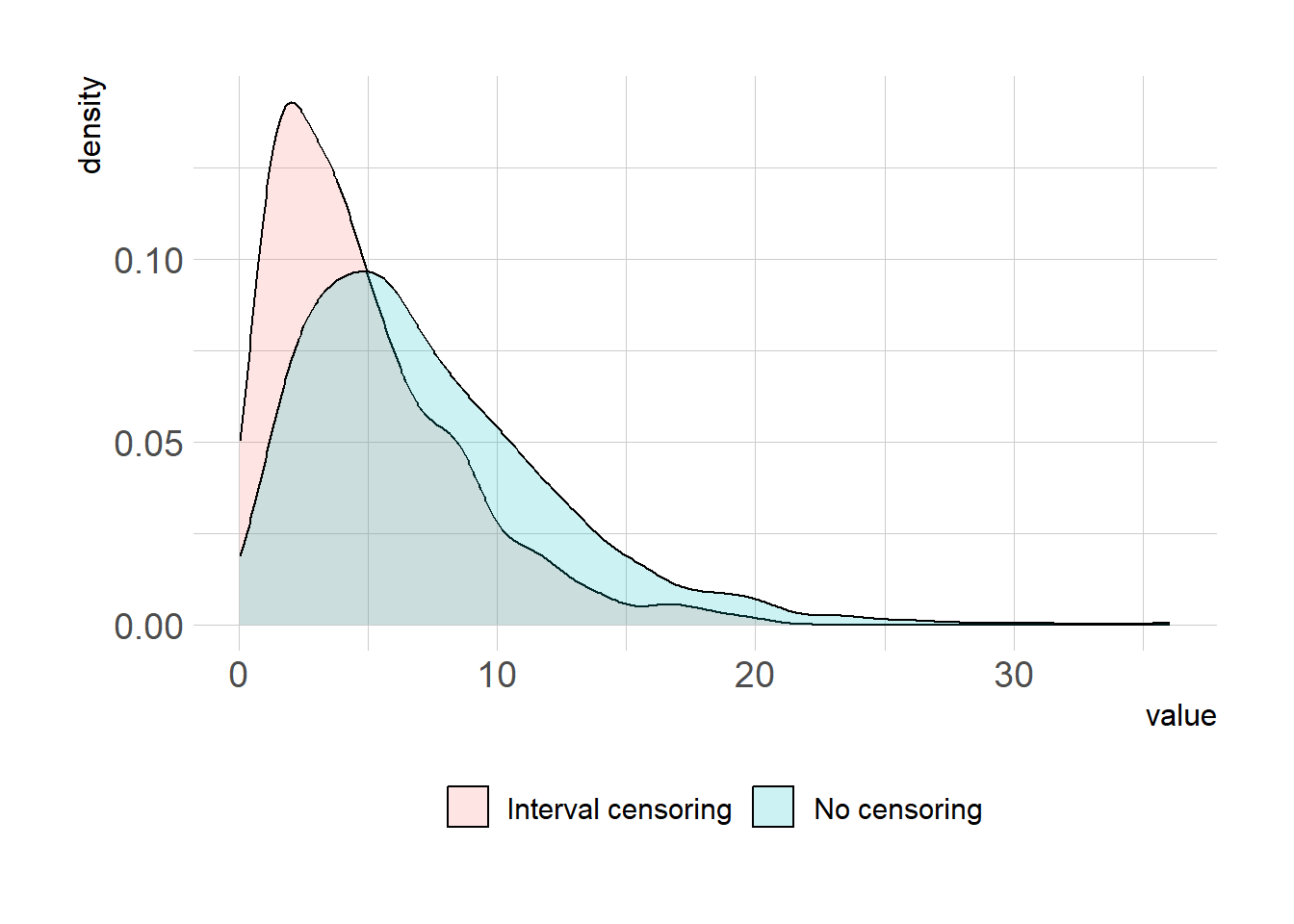
x1 <- rgamma(1e3, shape=res1$par[[1]], scale=res1$par[[2]])
x2 <- rgamma(1e3, shape=res2$par[[1]], scale=res2$par[[2]])
summary(x1)

   Min. 1st Qu.  Median    Mean 3rd Qu.    Max. 
 0.1677  3.7743  6.2386  7.3706 10.0134 36.0535 

summary(x2)

    Min.  1st Qu.   Median     Mean  3rd Qu.     Max. 
 0.05973  2.01266  3.88932  4.85497  6.77875 20.17723 

df = data.frame(model=rep(c("No censoring", "Interval censoring"), each=1e3), val=c(x1,x2))

library(ggplot2)
theme_set(hrbrthemes::theme_ipsum_rc(base_size=14, subtitle_size=16, axis_title_size=12))

df |> ggplot(aes(x=val, fill=model))+
  geom_density(alpha=0.2) +
  labs(x="value", y="density")+
  theme(legend.position = "bottom", 
        legend.title = element_blank())