Importance sampling

Importance sampling

Importance sampling is a Monte Carlo method for evaluating properties of a particular distribution, while only having samples generated from a different distribution than the distribution of interest.

Suppose we want to compute the expectation of an arbitrary function \(f\) of a random variable \(Y\), which is distributed according to the distribution \(p\): \[ E_p[f(Y)] := \int f(y) p(y) dy\]

In case the integration becomes difficult, we can use a Monte Carlo method. \[ E^{MC} := \frac{1}{N} \sum_{i=1}^N f(y^{(i)})\] By the law of large numbers, this estimate will almost surely converge to the true value as the number \(N\) of particles (i.e., sampled values) increases.

Although this appears straightforward, sampling from the target distribution, \(p\) is not always possible or efficient. Importance sampling bypasses this difficulty by sampling particles from an arbitrary “instrumental distribution” \(q\) and weighting the particles by accounting for they were sampled from \(q\) but not from \(p\).

Importance sampling fundamental identity

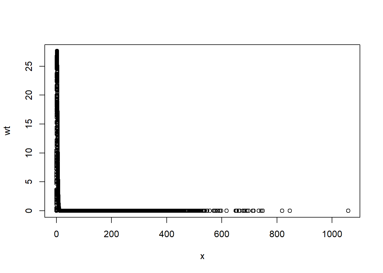
\[ E_p[f(Y)] := \int \frac{f(y)}{q(y)} q(y) p(y) dy = E_q[w(Y) f(Y)]\] where we define the importance weight \(w(y) = \frac{p(y)}{q(y)}\)

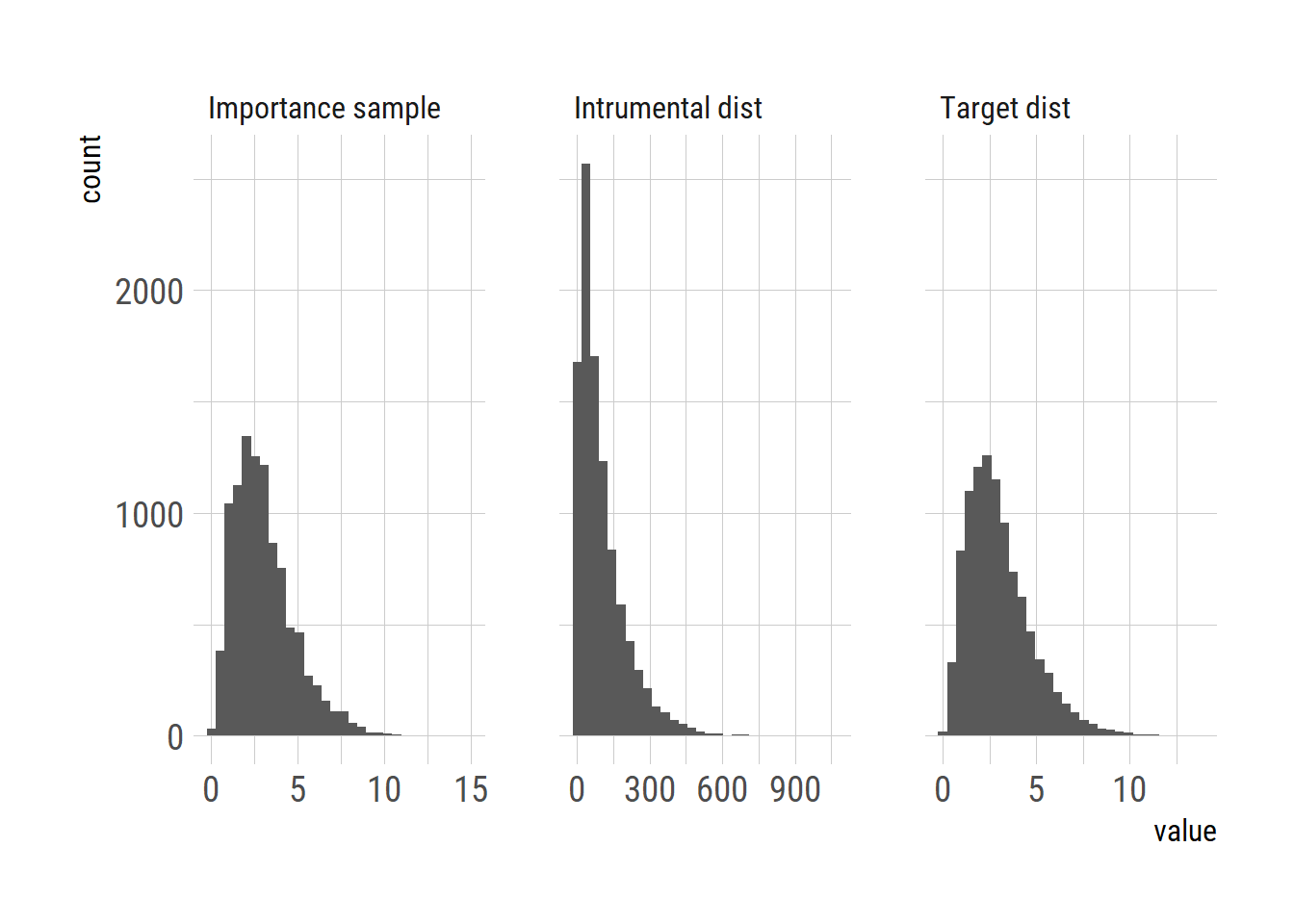
Let’s see an example in which we create Gamma-distributed sample from the exponentially distributed sample.

set.seed(42)
r <- 0.01 # low rate for a wide coverage
x <- rexp(1e4, rate=r)
# dgamma(x, shape=3, rate=1) target distribution
wt = dgamma(x, shape=3, rate=1) / dexp(x, rate=r)

plot(x, wt)

W = wt/sum(wt)

ids <- sample(1:length(x), prob=W, replace=T)
newx <- x[ids]
d <- data.frame(wt=wt, x=x, W=W)
d <- d[order(x),]
y = rgamma(length(x), shape=3, rate=1)

d <- data.frame(mean_exp=mean(x),
                sum_wt_x=sum(W*x),
                mean_important=mean(newx),
                true_mean = mean(y))

d

  mean_exp sum_wt_x mean_important true_mean
1 100.6511  3.01221       3.046269  3.035831

df <- data.frame(name=rep(c("Target dist","Intrumental dist","Importance sample"), each=1e4), 
                 value=c(y,x,newx))
library(ggplot2)
theme_set(hrbrthemes::theme_ipsum_rc(base_size=14, subtitle_size=16, axis_title_size=12))
extrafont::loadfonts()
ggplot(df)+
  geom_histogram(aes(x=value))+
  facet_wrap(~name, nrow=1, scales="free_x")

# ggsave("importance_sampling.png", gg, units="in", width=3.4*2, height=2.7*2)