Multinomial distribution

A simple particle filter in R

When implementing a model of stochastic disease transmission, one has to deal with a situation in which multiple events are possible. For example, susceptible people may become infected, remain susceptible, or die from other causes. In R, one could use rmultinorm as long as one can assign a probability for each event. Here, however, we implement a function from scratch. One way is to follow the approach of Aaron King, author of the pomp package. His method is implemented in C and I adapted it to R and C++ while removing many of its auxiliary functions (e.g., checking the validity of the inputs).

reulermultinom2 <- function (m=2, size, rate, dt) {
  trans <- matrix(NA, nrow=m, ncol=length(rate))
  p <- 0.0 # total event rate
  if ((size < 0.0) | (dt < 0.0) | (floor(size+0.5) != size)) {
    for (k in seq_along(rate)) {
      trans[k] = NaN
    }
    return(trans)
  }
  if (sum(rate < 0.0) > 0){
    stop("Negative rates  are not allowed")
  }
  else {
    p <- sum(rate)
  }
  if (p > 0.0) {
    for (i in 1:m) {
      tmpsize <- rbinom(1, size = size, prob = (1-exp(-p*dt))) # total number of events
      tmpp <- p
      for (k in 1:(length(rate)-1)) {
        trans[i, k] = rbinom(1, tmpsize, rate[k]/tmpp)
        tmpsize = tmpsize - trans[i, k];
        tmpp = tmpp - rate[k];
      }
      trans[i, length(rate)] = tmpsize;
    }    
  } 
  
  return(trans)
}

Let’s compare it with the original function provided in the pomp package

x <- t(pomp::reulermultinom(1e5, 100, rate=c(1,2), dt=0.05))
y <- reulermultinom2(1e5, 100, rate=c(1,2), dt=0.05)
xy <- as.data.frame(cbind(x, y))
names(xy) <- c("pomp_var1", "pomp_var2", "var1", "var2")
apply(xy, 2, summary)

        pomp_var1 pomp_var2    var1     var2
Min.      0.00000   0.00000  0.0000  0.00000
1st Qu.   3.00000   7.00000  3.0000  7.00000
Median    4.00000   9.00000  4.0000  9.00000
Mean      4.64097   9.27939  4.6419  9.28399
3rd Qu.   6.00000  11.00000  6.0000 11.00000
Max.     16.00000  25.00000 15.0000 24.00000

The speed difference is quite substantial.

library(microbenchmark)
microbenchmark(pomp::reulermultinom(100, 100, rate=c(1,2), dt=0.05), reulermultinom2(100, 100, rate=c(1,2), dt=0.05))

Unit: microseconds
                                                      expr     min       lq
 pomp::reulermultinom(100, 100, rate = c(1, 2), dt = 0.05)  39.702  41.4505
      reulermultinom2(100, 100, rate = c(1, 2), dt = 0.05) 377.301 384.9005
      mean  median       uq      max neval cld
  48.18708  43.651  48.0015   92.801   100  a 
 561.12002 401.851 641.1015 6275.101   100   b

Rewrite the function in C++ using Rcpp.

Rcpp::cppFunction("NumericMatrix reulermultinom_cpp(int m, double size, NumericVector rate, double dt) {
  int ncol = rate.size();
  NumericMatrix trans(m, ncol);
  double p = sum(rate); //total event rate
  for (int i = 0; i < m; i++) { 
    double tmpp = p;
    double tmpsize = R::rbinom(size, (1-exp(-tmpp*dt))); // total number of events
    for (int k = 0; k < (ncol-1); k++) {
      double tr = R::rbinom(tmpsize, rate(k)/tmpp);
      trans(i, k) = tr;
      tmpsize = tmpsize - trans(i, k);
      tmpp = tmpp - rate(k);
    }
    trans(i, (ncol-1)) = tmpsize;
  }    
  return(trans);
}")

library(microbenchmark)
microbenchmark(pomp::reulermultinom(1e5, 100, rate=c(1,2), dt=0.05), reulermultinom_cpp(1e5, 100, rate=c(1,2), dt=0.05))

Unit: milliseconds
                                                        expr     min       lq
 pomp::reulermultinom(1e+05, 100, rate = c(1, 2), dt = 0.05) 24.9228 27.61285
   reulermultinom_cpp(1e+05, 100, rate = c(1, 2), dt = 0.05) 23.9839 25.87615
     mean   median      uq      max neval cld
 51.27772 41.71065 66.0408 131.8367   100   a
 51.02618 43.38275 67.6930 120.4940   100   a

x <- t(pomp::reulermultinom(1e5, 100, rate=c(1,2), dt=0.05))
y <- reulermultinom_cpp(1e5, 100, rate=c(1,2), dt=0.05)
xy <- as.data.frame(cbind(x, y))
names(xy) <- c("pomp_var1", "pomp_var2", "var1", "var2")
apply(xy, 2, summary)

        pomp_var1 pomp_var2     var1     var2
Min.       0.0000   0.00000  0.00000  0.00000
1st Qu.    3.0000   7.00000  3.00000  7.00000
Median     4.0000   9.00000  4.00000  9.00000
Mean       4.6498   9.28149  4.64416  9.28147
3rd Qu.    6.0000  11.00000  6.00000 11.00000
Max.      17.0000  22.00000 15.00000 24.00000

library(tidyr)
xy |> pivot_longer(cols=1:4, names_to="var") -> xylong
library(ggplot2)
theme_set(hrbrthemes::theme_ipsum_rc(base_size=14, subtitle_size=16, axis_title_size=12))
extrafont::loadfonts()
ggplot(xylong)+
  geom_violin(aes(x=var, y=value))+
  facet_wrap(~var, nrow=1, scales="free_x")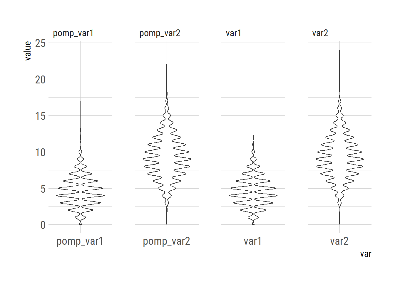

# ggsave("multinomial.png", gg, units="in", width=3.4*2, height=2.7*2)