Estimating serial interval: doubly interval-censored data

We start simple. Our task is to estimate parameters of a probability density function used to model the serial interval. Suppose dates of onsets of infectors, \(A\), and infectees, \(B\), are given as specific dates. Then the likelihood function for the serial interval may be written down as follows:
\[\mathcal{L}(X;\theta) = \prod_{i=1}^{n} f_{\theta}(B_i - A_i)\], where \(f\) is the probability density function for the serial interval with the unknown parameters, \(\theta\).

Now suppose that the dates of symptom onset of the infectors are given as intervals. We can use the following argument also for the case where dates of symptom onset of the infectees are given as intervals. In this case, the above likelihood function may be modified as follows:

\[\mathcal{L}(X;\theta) = \prod_{i=1}^{n} \int_{A^L_i}^{A^R_i} f_{\theta}(B_i-a) ~\text{d}a\] , where \(A^L, A^R, B\) present the times for lower end and upper bound on the potential dates of symptom onset of the infector, and the symptom onset time of the infectee, respectively.

Now suppose that both the dates of onset of the infectors and infectees are given as intervals. This is so called the doubly interval-censored data discussed by Reich et al 2009. The likelihood function may be given as follows:

\[\mathcal{L}(X;\theta,\lambda) = \prod_{i=1}^{n} \int_{A^L_i}^{A^R_i} \int_{B^L_i}^{B^R_i} h_{\lambda}(a) f_{\theta}(b-a) ~\text{d}b \text{d}a\] , where \(A^L, A^R, B^L, B^R\) present the times for left and right boundaires on the possible onset times of the infector, \(A\), and the infectee, \(B\), respectively. \(h_{\lambda}(x)\) represents the probability density function for the time of symptom onset of the infector, which we assume follows a uniform distribution.

More detailed analyses of doubly interval-censored data were discussed by Reich et al 2009. The same concept has recently been applied to estimation of serial interval of CVODI-19 by Nishiura et al. 2020.

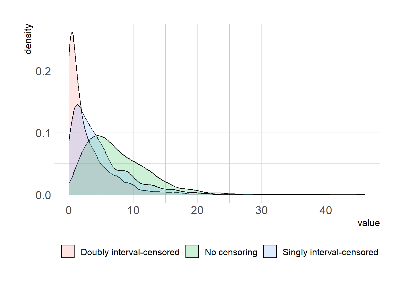
In the following codes, we create the fake data set and add intervals such that the serial intervals may become shorter.

set.seed(42)
n <- 100
shape_true <- 2.2
scale_true <- 3.3

onset_infector <- sample(20:30, size=n, replace=TRUE)
onset_infectee <- onset_infector + rgamma(n, shape=shape_true, scale=scale_true)
nll <- function(parms, x) -sum(dgamma(x, shape=parms[[1]], scale=parms[[2]], log=TRUE))
res1 = optim(par=c(1,2), fn=nll, x=onset_infectee - onset_infector, method = "Nelder-Mead",
            control = list(maxit=2e4, reltol=1e-15))

# singly interval-censored data
tau <- sample(1:5, n, replace=TRUE)
AL <- onset_infector 
AR <- onset_infector + 2*tau # this will lead to shorter serial interval

nll_single_censor <- function(parms, AL, AR, B){
  -sum(log(pgamma(B-AL, shape=parms[[1]], scale=parms[[2]]) - pgamma(B-AR, shape=parms[[1]], scale=parms[[2]])))
}

res2 = optim(par=c(1,2), fn=nll_single_censor, AL=AL, AR=AR, 
             B=onset_infectee, method="Nelder-Mead",
            control = list(maxit=2e4, reltol=1e-15))

# doubly interval-censored data
BL <- onset_infectee - 2*tau # this will lead to even shorter serial interval
BR <- onset_infectee

nll_double_censor <- function(parms, AL, AR, BL, BR){
  -sum(log(dunif(AL, min=AL, max=AR)*(pgamma(BR-AL, shape=parms[[1]], scale=parms[[2]]) - pgamma(BL-AR, shape=parms[[1]], scale=parms[[2]]))))
}

res3 = optim(par=c(1,2), fn=nll_double_censor, AL=AL, AR=AR,
             BL=BL, BR=BR, method="Nelder-Mead",
            control=list(maxit=2e4, reltol=1e-15))

x1 <- rgamma(1e3, shape=res1$par[[1]], scale=res1$par[[2]])
x2 <- rgamma(1e3, shape=res2$par[[1]], scale=res2$par[[2]])
x3 <- rgamma(1e3, shape=res3$par[[1]], scale=res3$par[[2]])
summary(x1)

   Min. 1st Qu.  Median    Mean 3rd Qu.    Max. 
 0.1677  3.8165  6.4303  7.5411 10.3268 36.0535 

summary(x2)

    Min.  1st Qu.   Median     Mean  3rd Qu.     Max. 
 0.03203  1.37089  3.37988  4.70497  6.48863 38.89572 

summary(x3)

    Min.  1st Qu.   Median     Mean  3rd Qu.     Max. 
 0.00001  0.36330  1.48009  2.92934  4.04038 46.12810 

df = data.frame(model=rep(c("No censoring", "Singly interval-censored",
                            "Doubly interval-censored"), each=1e3),
                val=c(x1,x2, x3))

library(ggplot2)
theme_set(hrbrthemes::theme_ipsum_rc(base_size=14, subtitle_size=16, axis_title_size=12))

df |> ggplot(aes(x=val, fill=model))+
  geom_density(alpha=0.2) +
  labs(x="value", y="density")+
  theme(legend.position = "bottom", 
        legend.title = element_blank())

# ggsave("double_interval_censor.png", gg, units="in", width=3.4*2, height=2.7*2)