Mass-action assumption: density- vs. frequency-dependent transmission

Density-dependent vs. frequency-dependent transmission

In models of transmission of directly transmitted pathogens, e.g., COVID-19, the transmission is assumed to occur via so-called mass action principle. It means the rate of newly infected people per unit area, per unit of time is proportional to the product between the numbers (or densities) of susceptible and infectious individuals. The term appears to be first coined by Hamer in 1906 in his paper. However, as indicated by McCallum, there have been some confusion over using the term, mass action. The confusion is around that mass action principle may be implemented in the manner of frequency-dependent or density-dependent transmission.

In the density-dependent transmission scenario, the rate of change in the number or density of infected individual can be implemented as follows:

\[\mathrm{d}I = \beta^* SI - \gamma I\].

In the frequency-dependent scenario, arguably more widely adopted one, the rate of change in the number or density of infected individual can be implemented as follows:

\[\mathrm{d}I = \beta SI/N - \gamma I\] Two formulations have different implications. The most notable difference is that there is a threshold density, \(N_T\) in the density-dependent formulation whereas the second model leads to the basic reproduction ratio, \(R_0\), is derived from frequency-dependent. Of course, it is straightforward to interchange between the two types of models.

Both \(\beta^*\) and \(\beta\) are transmission coefficients but their unit are different. In the frequency-dependent formulation, \(\beta\) can mean the number of transmissions per unit of time for an infected individual when it contacts with susceptible individuals. Therefore, the whole term, \(\beta I S/N\), could mean that the number of newly infected individuals per unit of time. For density-dependent formulation, \(\beta^*\) can mean the number of transmissions per unit of density per unit of time for an infected individual. The whole term \(\beta^* I S\) can then mean the density of newly infected individuals per unit of time.

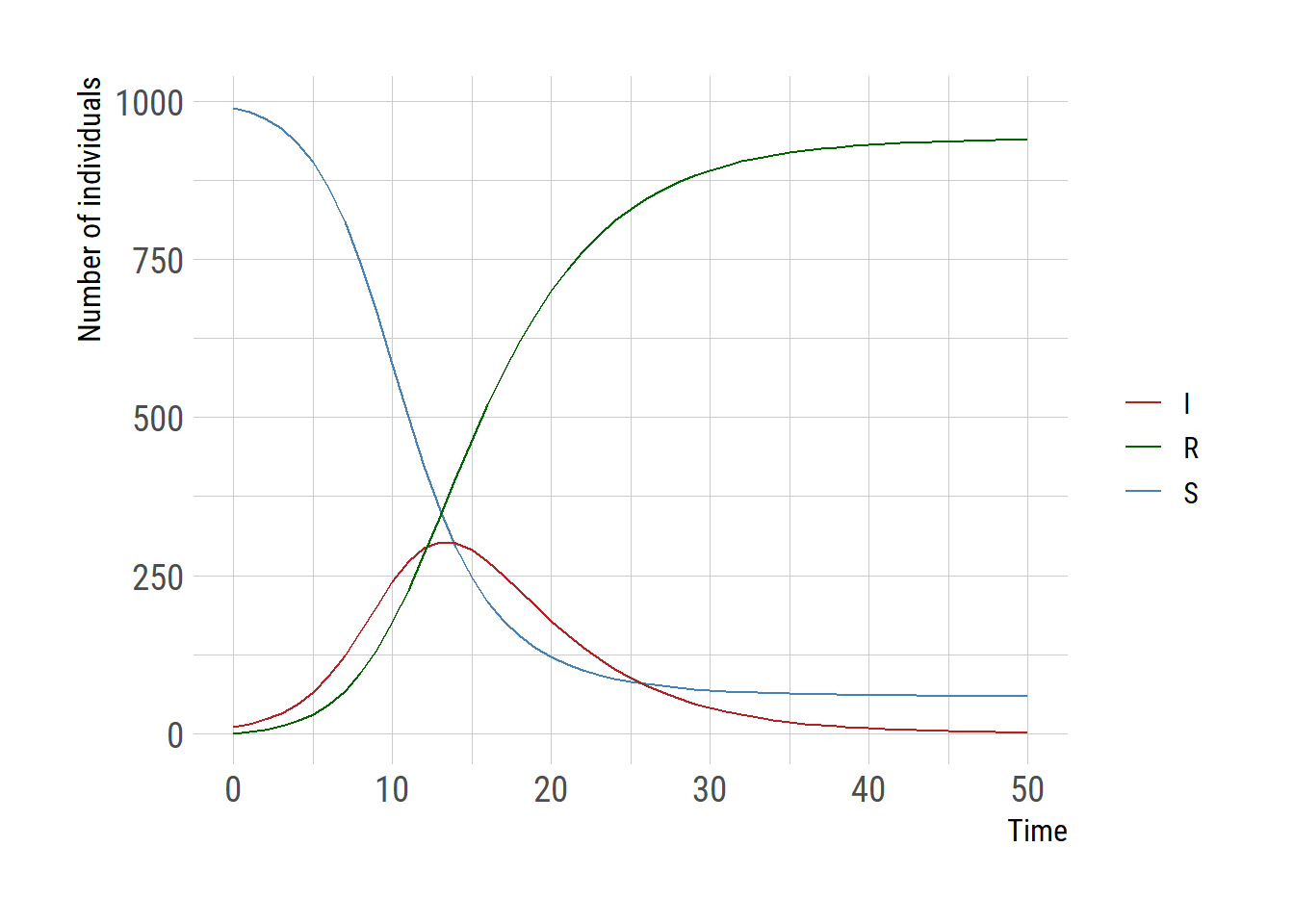
Now let’s implement a simple SIR model in two different formulations.

Density-dependent transmission

sir_den <- function(t, u, p){
  new_Istar = p[["beta_star"]]*u[1]*u[2]
  du1 <- - new_Istar
  du2 <- + new_Istar - p[["gamma"]]*u[2]
  du3 <- + p[["gamma"]]*u[2]
    
  return(list(c(du1,du2,du3))) 
}

library(deSolve)
pop = 1000
I0 = 10
u0 <- c(pop - I0, I0, 0)
tspan <- seq(from=0, to=50)
p <- c(beta_star=0.0006, gamma=0.2)

outdf <- as.data.frame(ode(y=u0, times=tspan, func=sir_den, parms=p))

library(ggplot2)
extrafont::loadfonts("win", quiet=TRUE)
theme_set(hrbrthemes::theme_ipsum_rc(base_size=14, subtitle_size=16, axis_title_size=12))

ggplot(outdf,aes(x=time))+
  geom_line(aes(y=`1`, color="S")) +
  geom_line(aes(y=`2`, color="I")) +
  geom_line(aes(y=`3`, color="R")) +
  scale_color_manual("",values=c("S"="steelblue","I"="firebrick",
                              "R"="darkgreen"))+
  labs(y="Number of individuals", x="Time", color="")

# threshold host population size
Nt = p["gamma"] / p["beta_star"]
# R0 can be computed through N/Nt
R0 = pop/Nt

final_epidemic_size <- function(R0 = 2) {
  y = function(x) x - 1 + exp(-R0*x)
  final_size <- uniroot(y, interval=c(1e-6,1-1e-6))$root

  return(final_size)

}
round(pop*final_epidemic_size(R0=R0), digits=2)

[1] 940.48

round(tail(outdf, 1)$`3`, digits=2)

[1] 939.32

Frequency-dependent formulation

sir_freq <- function(t, u, p){
  new_I = p[["beta"]]*u[1]*u[2]/sum(u)
  du1 <- - new_I
  du2 <- + new_I - p[["gamma"]]*u[2]
  du3 <- + p[["gamma"]]*u[2]
    
  return(list(c(du1,du2,du3))) 
}

library(deSolve)
pop = 1000
I0 = 10
u0 <- c(pop - I0, I0, 0)
tspan <- seq(from=0, to=50)
p <- c(beta=0.6, gamma=0.2)

outdf <- as.data.frame(ode(y=u0, times=tspan, func=sir_freq, parms=p))

ggplot(outdf,aes(x=time))+
  geom_line(aes(y=`1`, color="S")) +
  geom_line(aes(y=`2`, color="I")) +
  geom_line(aes(y=`3`, color="R")) +
  scale_color_manual("",values=c("S"="steelblue","I"="firebrick",
                              "R"="darkgreen"))+
  labs(y="Number of individuals", x="Time", color="")

# R0 threshold
(R0 = p[["beta"]] / p[["gamma"]])

[1] 3

round(pop*final_epidemic_size(R0=R0), digits=2)

[1] 940.48

round(tail(outdf, 1)$`3`, digits=2)

[1] 939.32