library(data.table)
d1 <- fread(here("data", "2008_Mossong_POLYMOD_participant_common.csv"))
d2 <- fread(here("data", "2008_Mossong_POLYMOD_contact_common.csv"))
library(dplyr)
# count the number of contacts for each participant using part_id variable
d2 |> group_by(part_id) |>
  summarize(contacts = n()) -> d2_contacts
d12 <- left_join(d1, d2_contacts, by="part_id")
# add household information
d3 <- fread(here("data", "2008_Mossong_POLYMOD_hh_common.csv"))
d123 <- left_join(d12, d3, by="hh_id")
# add day of week information
d4 <- fread(here("data", "2008_Mossong_POLYMOD_sday.csv"))
dat <- left_join(d123, d4, by="part_id")Mulitple regression: POLYMOD data
R
regression
contact
This post describes my attempt to reproduce Table 1 of the POLYMOD study (1), which is a large European study on social contacts and mixing patterns relevant to the spread of infectious diseases. Data were downloaded from Social Contact Data, which was hosted in zenodo (version 1.1). While I wasn’t successful at reproducing the table exatly but still wanted to document the processes that I went through. Potential reasons include: a) results of numerical computations vary depending on the system and the software and b) datasets that were analyzed might be slightly different because of the missing values.
Data preparation
Data manipulation
Categorize the age group into different 10 age groups: 0-4, 5-9, 10-14, 15-19, and 20 to 70 by 10 years and 70 and above
classify_age <- function(d){
  d$age_grp <- 99
  for (i in 1:nrow(d)) {
    if(!is.na(d$part_age[i])){
      if(d$part_age[i] < 5){
        d$age_grp[i] <- 0
      }
      else if (d$part_age[i] >= 5 && d$part_age[i] < 20){
        for(j in 1:3){
          if(d$part_age[i] >= 5*j && d$part_age[i] < (5*j+5)){
            d$age_grp[i] <- j
          }
        }
      }
      else if (d$part_age[i] >= 20 && d$part_age[i] < 70){
        for (k in 1:5){
          if (d$part_age[i] >= (10+10*k) && d$part_age[i] < (20+10*k)){
            d$age_grp[i] <- k+3
          }
        }
      }
      else {
        d$age_grp[i] <- 9
      }
    }
  }
  d
}

dat <- classify_age(dat)
Visualize the distribution of the number of contacts
library(ggplot2)
dat |> ggplot(aes(x=contacts)) +
  geom_histogram(binwidth=5)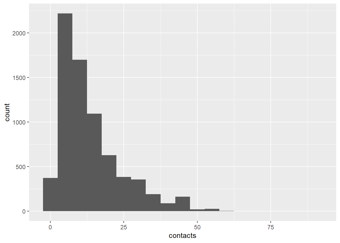
Compare the number of participants by age group (the third column)
dat |>
  group_by(age_grp) |>
  summarize(npart=n(),
            avg_contacts = round(sum(contacts, na.rm=T) / npart, digits=2)) -> dat_ag

dat_ag$npart_true <- c(660,661,713,685,879,815,908,906,728,270,65)
dat_ag$avg_contacts_true <- c(10.21,14.81, 18.22,17.58,13.57,14.14,13.83,12.30,9.21,6.89,9.63)
dat_ag
# A tibble: 11 횞 5
age_grp npart avg_contacts npart_true avg_contacts_true
<dbl> <int> <dbl> <dbl> <dbl>
1 0 660 10.2 660 10.2
2 1 661 14.8 661 14.8
3 2 713 18.2 713 18.2
4 3 685 17.6 685 17.6
5 4 879 13.6 879 13.6
6 5 815 14.1 815 14.1
7 6 908 13.8 908 13.8
8 7 906 12.3 906 12.3
9 8 728 9.21 728 9.21
10 9 270 6.89 270 6.89
11 99 65 9.63 65 9.63Categorize the household size
classify_hh <- function(d){
  d$hh_size_grp <- ifelse(d$hh_size > 4, 5, ifelse(!is.na(d$hh_size), d$hh_size, 99))
  d
}
dat <- classify_hh(dat)
# data.table::fwrite(dat, "data/POLYMOD_2017.csv")
Make categorical variables factor for regression
# dat <- data.table::fread("data/POLYMOD_2017.csv")
# set the categorical variables as factor for regression
dat$age_grp <- as.factor(dat$age_grp)
dat$hh_size_grp <- as.factor(dat$hh_size_grp)
dat$gender <- ifelse(dat$part_gender=="M", 0, ifelse(dat$part_gender=="F", 1, 99))
dat$gender <- as.factor(dat$gender)
dat$dayofweek <- as.factor(dat$dayofweek)
# dat <- dat[complete.cases(dat),]
# data.table::fwrite(dat, "data/POLYMOD_2017_gender_modified.csv")
Linear regression
While I will eventually use the negative binomial regresssion, I tried linear regression with which my colleague who uses Stata is familiar.
library(MASS)
# to remove missing values
dat <- dat[complete.cases(dat),]

m <- lm(contacts ~ age_grp + gender + hh_size_grp + country + dayofweek, data = dat)
summary(m)
Call:
lm(formula = contacts ~ age_grp + gender + hh_size_grp + country +
    dayofweek, data = dat)

Residuals:
    Min      1Q  Median      3Q     Max
-21.204  -6.129  -1.718   3.880  80.052

Coefficients:
             Estimate Std. Error t value Pr(>|t|)
(Intercept)    2.5978     0.7067   3.676 0.000239 ***
age_grp1       4.1734     0.5168   8.076 7.80e-16 ***
age_grp2       7.7402     0.5072  15.262  < 2e-16 ***
age_grp3       7.4715     0.5117  14.602  < 2e-16 ***
age_grp4       4.6392     0.4934   9.402  < 2e-16 ***
age_grp5       4.5177     0.4981   9.070  < 2e-16 ***
age_grp6       4.1732     0.4863   8.581  < 2e-16 ***
age_grp7       3.2931     0.5024   6.554 5.99e-11 ***
age_grp8       1.2232     0.5501   2.224 0.026206 *
age_grp9      -1.1332     0.7209  -1.572 0.115997
gender1        0.1746     0.2216   0.788 0.430686
gender99       2.0543     2.9437   0.698 0.485271
hh_size_grp2   0.8352     0.4244   1.968 0.049133 *
hh_size_grp3   1.0815     0.4498   2.404 0.016231 *
hh_size_grp4   2.7105     0.4549   5.959 2.67e-09 ***
hh_size_grp5   3.9035     0.4951   7.884 3.64e-15 ***
countryDE     -3.5686     0.4315  -8.270  < 2e-16 ***
countryFI     -0.5878     0.4519  -1.301 0.193398
countryGB     -0.3451     0.4530  -0.762 0.446204
countryIT      7.5967     0.4691  16.194  < 2e-16 ***
countryLU      5.0942     0.4500  11.321  < 2e-16 ***
countryNL      2.9129     0.6754   4.313 1.63e-05 ***
countryPL      4.0530     0.4489   9.029  < 2e-16 ***
dayofweek1     3.7578     0.4317   8.705  < 2e-16 ***
dayofweek2     4.5691     0.4244  10.767  < 2e-16 ***
dayofweek3     4.4291     0.4336  10.214  < 2e-16 ***
dayofweek4     4.5608     0.4277  10.664  < 2e-16 ***
dayofweek5     4.7862     0.4234  11.303  < 2e-16 ***
dayofweek6     1.6347     0.4414   3.703 0.000214 ***
---
Signif. codes:  0 '***' 0.001 '**' 0.01 '*' 0.05 '.' 0.1 ' ' 1

Residual standard error: 9.271 on 7040 degrees of freedom
Multiple R-squared:  0.2383,    Adjusted R-squared:  0.2352
F-statistic: 78.64 on 28 and 7040 DF,  p-value: < 2.2e-16
NegBin regression
Negative binomial regression was modeled using MASS::glm.nb function
library(MASS)
m1 <- glm.nb(contacts ~ age_grp, data = dat)
summary(m1)
Call:
glm.nb(formula = contacts ~ age_grp, data = dat, init.theta = 2.349538851,
    link = log)

Coefficients:
            Estimate Std. Error z value Pr(>|z|)
(Intercept)  2.33297    0.02847  81.959  < 2e-16 ***
age_grp1     0.34973    0.03963   8.826  < 2e-16 ***
age_grp2     0.57379    0.03861  14.862  < 2e-16 ***
age_grp3     0.53545    0.03908  13.702  < 2e-16 ***
age_grp4     0.28592    0.03733   7.660 1.86e-14 ***
age_grp5     0.31980    0.03780   8.460  < 2e-16 ***
age_grp6     0.29453    0.03707   7.946 1.93e-15 ***
age_grp7     0.18429    0.03716   4.959 7.09e-07 ***
age_grp8    -0.09048    0.03958  -2.286   0.0223 *
age_grp9    -0.38437    0.05435  -7.072 1.53e-12 ***
---
Signif. codes:  0 '***' 0.001 '**' 0.01 '*' 0.05 '.' 0.1 ' ' 1

(Dispersion parameter for Negative Binomial(2.3495) family taken to be 1)

    Null deviance: 8082.4  on 7068  degrees of freedom
Residual deviance: 7381.8  on 7059  degrees of freedom
AIC: 49343

Number of Fisher Scoring iterations: 1

              Theta:  2.3495
          Std. Err.:  0.0452

2 x log-likelihood: -49321.1310 exp(m1$coefficients)(Intercept) age_grp1 age_grp2 age_grp3 age_grp4 age_grp5
10.3085271 1.4186911 1.7749820 1.7082181 1.3309824 1.3768472
age_grp6 age_grp7 age_grp8 age_grp9
1.3424987 1.2023627 0.9134947 0.6808798 m5 <- glm.nb(contacts ~ age_grp + gender + hh_size_grp + country + dayofweek, data = dat)
summary(m5)
Call:
glm.nb(formula = contacts ~ age_grp + gender + hh_size_grp +
    country + dayofweek, data = dat, init.theta = 3.032960306,
    link = log)

Coefficients:
              Estimate Std. Error z value Pr(>|z|)
(Intercept)   1.733148   0.050127  34.575  < 2e-16 ***
age_grp1      0.320217   0.036004   8.894  < 2e-16 ***
age_grp2      0.513597   0.035093  14.635  < 2e-16 ***
age_grp3      0.512688   0.035437  14.468  < 2e-16 ***
age_grp4      0.359741   0.034520  10.421  < 2e-16 ***
age_grp5      0.343102   0.034802   9.859  < 2e-16 ***
age_grp6      0.313841   0.034051   9.217  < 2e-16 ***
age_grp7      0.253024   0.035267   7.175 7.25e-13 ***
age_grp8      0.048104   0.039074   1.231 0.218283
age_grp9     -0.211659   0.052694  -4.017 5.90e-05 ***
gender1       0.007832   0.015357   0.510 0.610050
gender99      0.077826   0.207001   0.376 0.706941
hh_size_grp2  0.098342   0.030472   3.227 0.001250 **
hh_size_grp3  0.117260   0.031984   3.666 0.000246 ***
hh_size_grp4  0.235206   0.032164   7.313 2.62e-13 ***
hh_size_grp5  0.323285   0.034725   9.310  < 2e-16 ***
countryDE    -0.345037   0.030616 -11.270  < 2e-16 ***
countryFI    -0.054068   0.031613  -1.710 0.087209 .
countryGB    -0.023021   0.031609  -0.728 0.466429
countryIT     0.488765   0.032064  15.244  < 2e-16 ***
countryLU     0.340195   0.030948  10.993  < 2e-16 ***
countryNL     0.219279   0.046632   4.702 2.57e-06 ***
countryPL     0.281896   0.030944   9.110  < 2e-16 ***
dayofweek1    0.278478   0.030363   9.172  < 2e-16 ***
dayofweek2    0.336024   0.029800  11.276  < 2e-16 ***
dayofweek3    0.328357   0.030383  10.807  < 2e-16 ***
dayofweek4    0.326135   0.029980  10.879  < 2e-16 ***
dayofweek5    0.365918   0.029655  12.339  < 2e-16 ***
dayofweek6    0.143777   0.031178   4.611 4.00e-06 ***
---
Signif. codes:  0 '***' 0.001 '**' 0.01 '*' 0.05 '.' 0.1 ' ' 1

(Dispersion parameter for Negative Binomial(3.033) family taken to be 1)

    Null deviance: 9903.4  on 7068  degrees of freedom
Residual deviance: 7310.7  on 7040  degrees of freedom
AIC: 47832

Number of Fisher Scoring iterations: 1

              Theta:  3.0330
          Std. Err.:  0.0626

2 x log-likelihood: -47771.7930 exp(m5$coefficients) (Intercept) age_grp1 age_grp2 age_grp3 age_grp4 age_grp5
5.6584394 1.3774273 1.6712925 1.6697736 1.4329588 1.4093123
age_grp6 age_grp7 age_grp8 age_grp9 gender1 gender99
1.3686718 1.2879141 1.0492799 0.8092407 1.0078631 1.0809342
hh_size_grp2 hh_size_grp3 hh_size_grp4 hh_size_grp5 countryDE countryFI
1.1033402 1.1244116 1.2651689 1.3816597 0.7081939 0.9473682
countryGB countryIT countryLU countryNL countryPL dayofweek1
0.9772421 1.6303023 1.4052212 1.2451789 1.3256406 1.3211173
dayofweek2 dayofweek3 dayofweek4 dayofweek5 dayofweek6
1.3993730 1.3886852 1.3856028 1.4418376 1.1546267 References
1.
Mossong J, Hens N, Jit M, Beutels P, Auranen K, Mikolajczyk R, et al. Social contacts and mixing patterns relevant to the spread of infectious diseases. PLOS Medicine. 2008;5(3):e74. doi:10.1371/journal.pmed.0050074