Learning ChatGPT 4: Universal Approximation Theorem

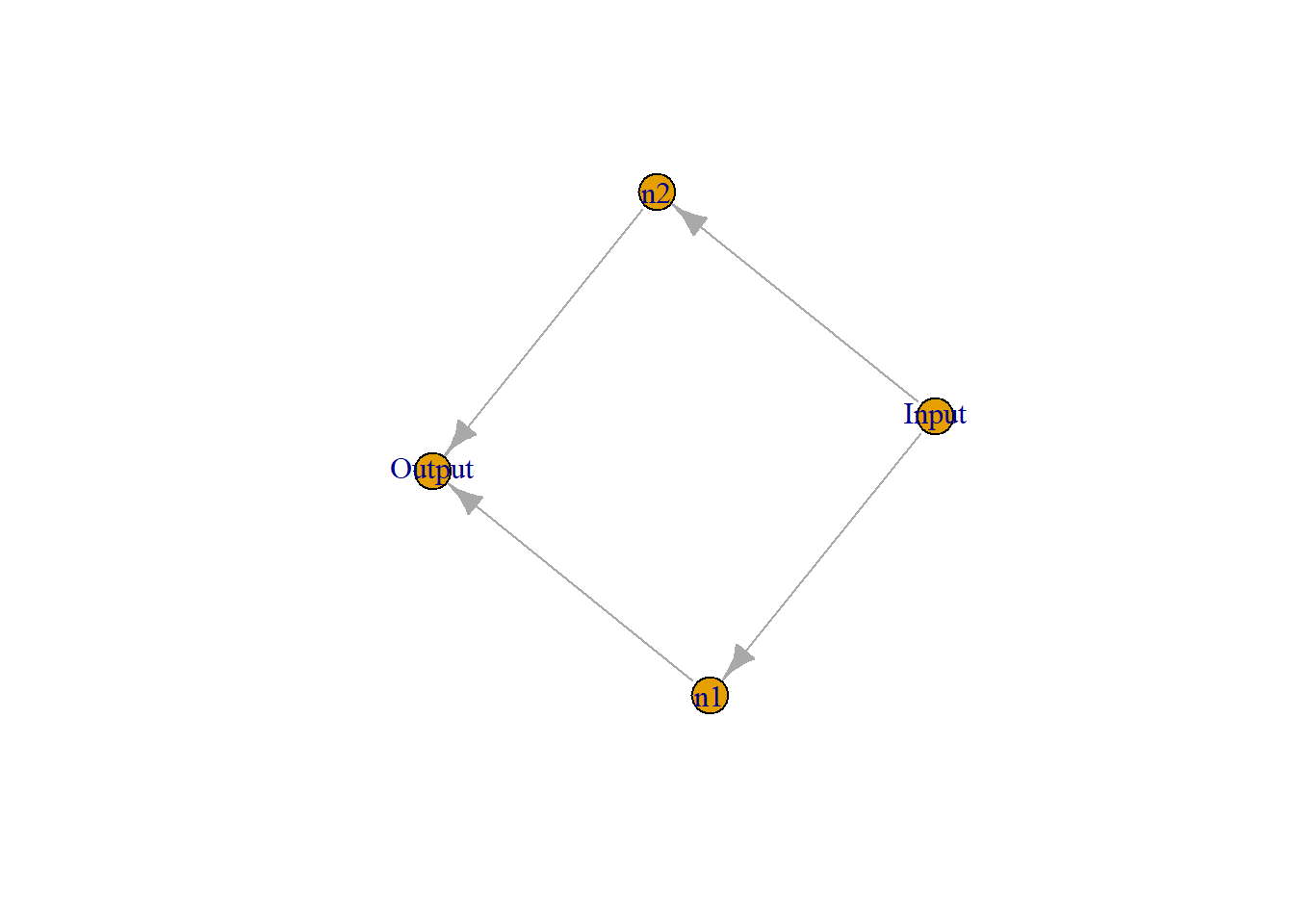
Neural networks can approximate any function according to the Universal Approximation Theorem. A more precise statement of the theorem is that neural networks with a single hidden layer can be used to approximate any continuous function to any desired precision by the e-book by Michael Nielsen. This e-book provides intuitive explanations about the proof. In what follows, I wrote what I was able to understand based on those materials and added a few R code chunks to supplement.

For a simple network with one hidden layer of two neurons, n1 and n2, what is being computed in a hidden neuron is \(\sigma(w x + b)\), where \(\sigma (z) \equiv 1/(1+e^{-z})\) is the sigmoid function. And what happens in the output neuron is \(w_{31} n1 + w_{32} n2 + b\). Here, \(w_{31} \text{and} w_{32}\) refer to weights that correspond to two neurons, n1 and n2, respectively.

The basic idea of the theorem is that weighted sum of outputs of neurons can approximate any functions. This can be visualized by studying a special case in which output from each neuron is close to a step function and weighted sum of a pair of step functions can create a bump of any height and width. With numerous those bumps, one can approximate any continuous function at any desired precision.

library(igraph)
plot(graph_from_literal(Input--+n1, Input--+n2, n1--+Output, n2--+Output))

In what follows, I will explain how a neural network can create a bump. Before that, let’s get familiar with what is being computed in a single neuron. In the following codes, some combination of weight, \(w\) , and bias, \(b\), generate a typical sigmoid function.

x <- seq(0, 1, 0.01)
w <- 20
b <- -5
plot(x, 1/(1+exp(-(w*x+b))), type="l", xlab="Input", ylab="n1")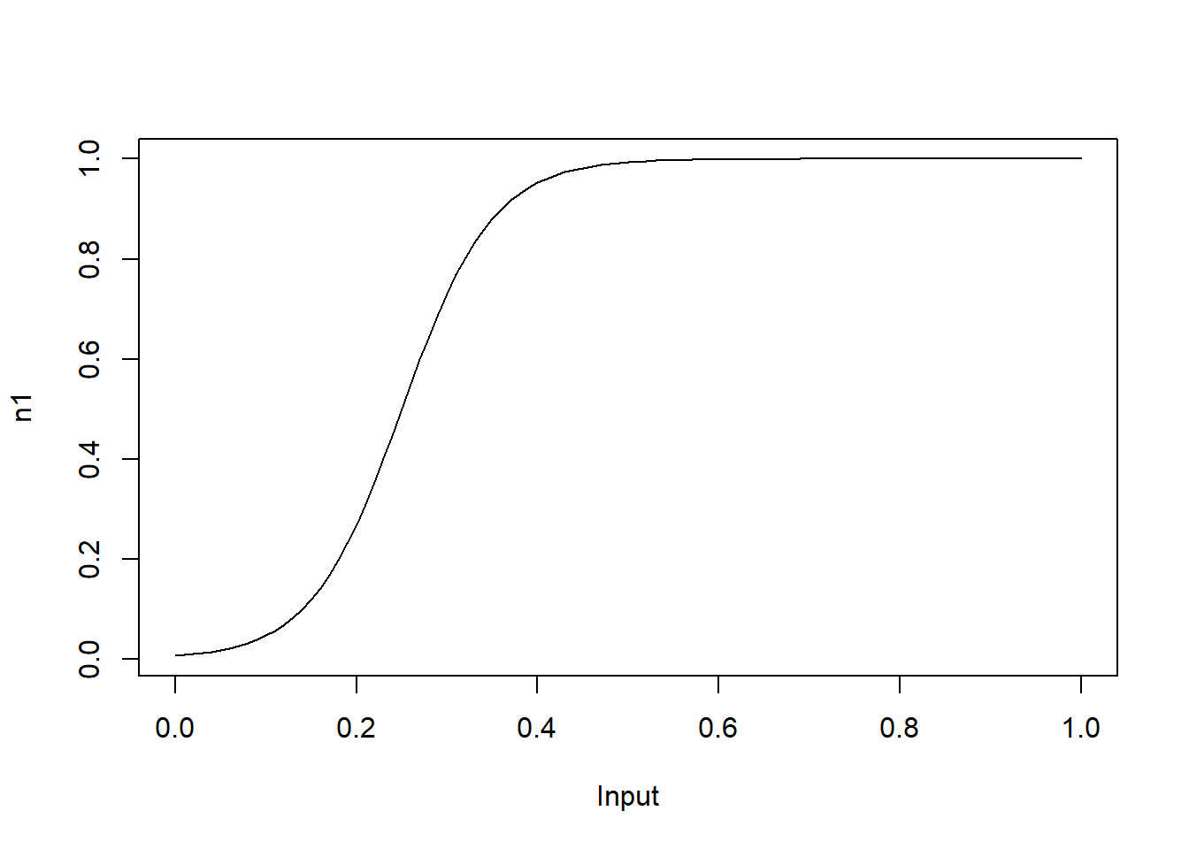

With high values for \(w\), the output becomes close to a step function and the change point occurs at \(-b/w\). For instance, let’s look at the plot for \(w=1000, b=-300\).

x <- seq(0, 1, 0.01)
w <- 1e3
b <- -300
plot(x, 1/(1+exp(-(w*x+b))), type="l", xlab="Input", ylab="n1")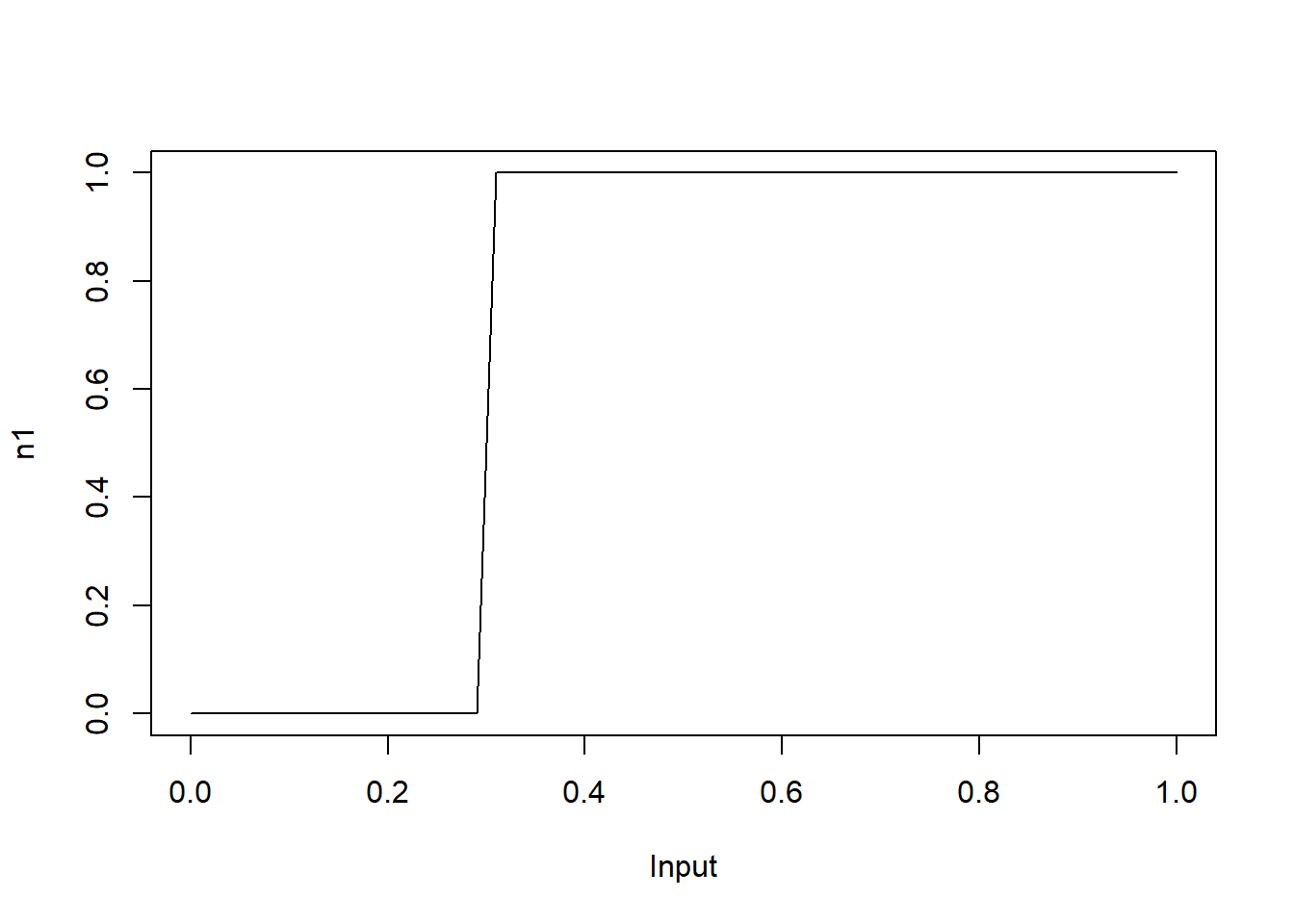

One can use the following codes to have a feel for how the weight and bias change the value in the neuron.

library(manipulate)
manipulate(
  plot(x, 1/(1+exp(-(w*x+b))), type="l", xlab="Input", ylab="n1"),
  w = slider(-1e3,1e3, initial = 20), 
  b = slider(-1e3,1e3, initial = -5))

Now let’s create another step function in which the change point occurs at 0.4

x <- seq(0, 1, 0.01)
w1 <- 1000
b1 <- -300
y1 <- 1/(1+exp(-(w1*x+b1)))
plot(x, y1, type="l")

w2 <- 1000
b2 <- -400
y2 <- 1 / (1+exp(-(w2*x+b2)))
lines(x, y2, col=2)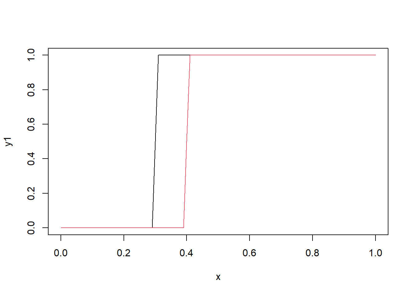

What happens in the Output node is \(\omega_{31} n1 + \omega_{32} n2 + b\). By setting \(w1\) and \(w2\) at different sign, we can create a bump.

w31 <- 1        
w32 <- -1       
b3 <- 0
plot(x, y2*w32 + y1*w31 + b3, type="l", xlab="x", ylab="Output")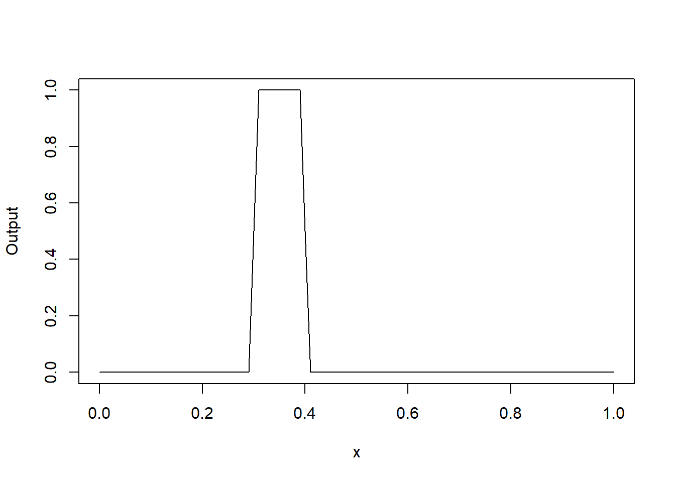

Again, one may use the following codes to have a feel for how two weights and the bias change the output in the Output.

manipulate(
  plot(x, y2*w32 + y1*w31 + b3, type="l", xlab="x", ylab="Output"),
  w31 = slider(-1e2,1e2, initial = 1), 
  w32 = slider(-1e2,1e2, initial = -1),
  b3 = slider(-1e2,1e2, initial = 0))